Figures & data
Table 1. Psycholinguistic properties of the 134 stimulus items. Mean and SD, median and range are reported, as calculated across items and for mosyllabic and disyllabic words separately.
Table 2. Averaged RT and naming accuracy values per semantic category, monosyllabic and dysillabic words (length), different groups based on PND, Word Frequency, and articulatory differences.
Figure 1. Object categories. A. Stimulus-locked data. Top panel. Cortical distribution (left hemisphere) of the above chance decoded activity specific to the object category condition (after controlling for visual features, including pixel information: see methods). Bottom panels: Time course of the above chance decoded activity in early visual cortex (left panel), posterior inferior/middle temporal cortex and posterior fusiform within the first 180 ms post-stimulus onset. B. Response-locked data. Top panel. Cortical distribution (left hemisphere) of the above chance decoded activity specific to the object category condition (after controlling for visual features, including pixel information: see methods). Bottom panels: Time course of the above chance decoded activity in inferior/middle temporal and frontal cortex linked to conceptual preparation before speech onset time.
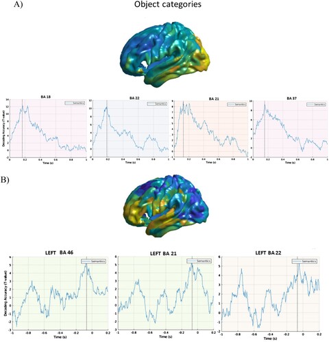
Figure 2. Word length. A. Stimulus-locked data. Top panel. Cortical distribution (left hemisphere) of the above chance decoded activity specific to the word length condition after controlling for word frequency. Bottom panel: Time course of the above chance decoded activity in the LIFG BA 44 and premotor cortex (BA 6), respectively within the first 200 ms and 100 ms post-stimulus onset. B. Response-locked data. Left panel. Cortical distribution (left hemisphere) of the above chance decoded activity specific to the word length condition. Right panel: Time course of the above chance decoded cortical activity in the LIFG BA 44 and the premotor cortex (BA 6) before speech onset: effects can be seen from about −800 before speech onset.
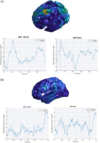
Figure 3. Phonological neighbourhood density. A. Stimulus-locked data. Top panel. Cortical distribution (left hemisphere) of the above chance decoded activity specific to the phonological neighbourhood density condition, after controlling for word frequency. Bottom panel: Time course of the above chance decoded activity in the LIFG BA 44, peaking around 100 ms post-stimulus onset and motor cortex, showing low levels of above chance decoding accuracy overall. B. Response-locked data. Top panel. Cortical distribution (left hemisphere) of the above chance decoded activity specific to the phonological neighbourhood density condition. Bottom panel: Time course of the above chance decoded activity in the LIFG BA 44 with no effects before speech onset. In motor cortex, a transient early effect was seen, around 800 ms before speech onset, which could not be seen in the stimulus-locked analyses.
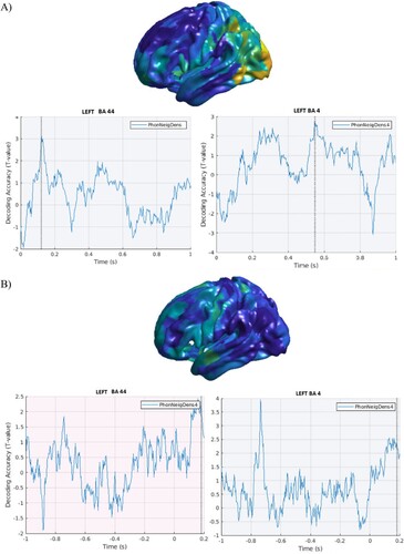
Figure 4. Place of articulation. A. Stimulus-locked data. Top panel. Cortical distribution of the above chance decoded activity specific to the Place of Articulation condition, after controlling for word frequency. Bottom panel: Time course of the above chance decoded activity in the LIFG BA 44, premotor and motor cortex. B. Response-locked data. Top panel. Cortical distribution (left hemisphere) of the above chance decoded activity specific to the Place of Articulation condition. Bottom panel: Time course of the above chance decoded activity in the LIFG BA 44 and motor cortex.
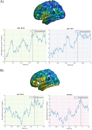
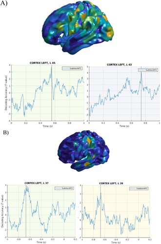
Figure 5. Word frequency. A. Stimulus-locked data. Top panel. Cortical distribution of the above chance decoded activity specific to word frequency in widespread brain regions. Bottom panel: Time course of the above chance decoded activity in the LIFG BA 45 and 43, with effects present within the first 600 ms post-stimulus onset. B. Response-locked data. Top panel. Cortical distribution of the above chance decoded activity specific to word frequency in widespread brain regions. Bottom panel: Time course of the above chance decoded activity in the LIFG BA 37 and BA 39, with peaks around −700 ms before speech onset.