Figures & data
Figure 1. Processing pipeline for the retrospective drift correction algorithm evaluated in this study. The main algorithm comprised of a DC drift correction and a 3D first-order drift correction.
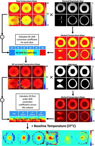
Table 1. Acquisition information of different scans applied in this study. Three sequences (referred as ACQ1, ACQ2, and ACQ3) in total were performed based on the experiment requirement. TE and TR represent echo time and repetition time, respectively.
Figure 2. T1-weighted images acquired along (A) and across (B) the ultrasound beam. Two fibre-optic temperature probes were used to validate MR thermometry during MR-HIFU hyperthermia exposures in a phantom. The dashed line in (A) depicts the centre of the plane where MR thermometry was performed during heating. The locations of two temperature probes are shown in (B). Zoomed-in view of the dashed square region in (B) is shown in (C), with the precise location of heating. The ultrasound beam was rapidly scanned along an 8-mm circular trajectory resulting in a uniform region of heating around probe 1.
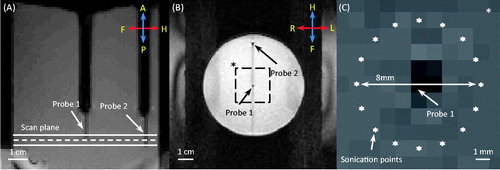
Figure 3. (A) T1-weighted image along the ultrasound beam axis shows the experimental set-up for performing hyperthermia in a rabbit model. A gel pad and a water tank were placed on top of the acoustic window of the clinical MR-HIFU system to elevate the animal to the location of the ultrasound focus. The conical water tank also maintained the body temperature of the animals. (B) T2-weighted image transverse to the beam axis (along the dashed line in A) shows the VX2 tumour and the location of heating. (C) The spatial temperature distribution measured midway during treatment shows localised heating within the target area, well maintained in the desired range of 41–43 °C.
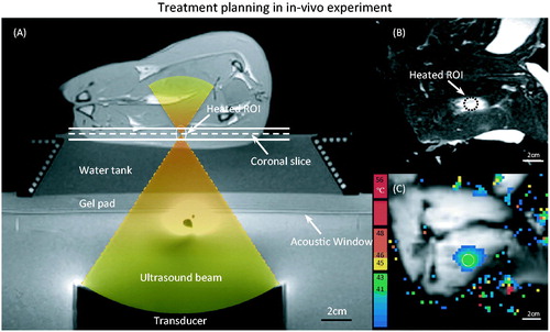
Figure 4. Scanner temperature and phase change under different thermometry sequence. (A) Temperature of the inner bore of the MRI increased at different rates during scanning depending on the gradient duty cycle of the sequence: echo-planar (EPI, upper curve) versus fast field echo (FFE, lower curve). The scan parameter and fan setting in the MR console were kept the same for two sequences. (B) Phase measurements acquired with MR thermometry (red and blue increasing curves) in an unheated phantom during scanning shows a monotonic change in phase. No significant temperature change was observed in the phantom (green and pink flat curves). The rate of change appears to be related to the gradient duty cycle and magnet heating.
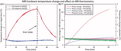
Figure 5. Zero- and first-order correction coefficients across all slices acquired in 3D first-order drift correction. (A) Zero-order coefficients over 60 min of scanning for an unheated phantom in the magnet. (B) The rate of change of the zero-order coefficient ranges from 1–2 °C/min over the first 30 min, with greater temporal variation over the first 10–15 min. (C) First-order drift correction coefficients (in plane and through plane) over 60 min for the same unheated phantom in the magnet. (D) The rate of change of the first-order coefficients also depicts more temporal variation in the first 10–15 min followed by steady monotonic variations.
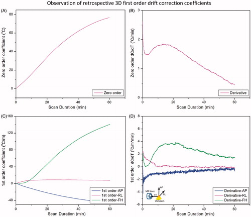
Figure 6. Effect of dynamic stabilisation, DC drift correction and pre-heating correction coefficients across all slices acquired in 3D first-order drift correction. F0 dynamic stabilisation and DC drift correction both reduce the magnitude (A) and rate of change (B) of the zero-order coefficient. DC drift correction was able to remove the noise introduced by dynamic stabilisation (B). Dynamic stabilisation alone was not enough to entirely remove the first-order variations along the AP direction (C), but coupled with the DC drift correction, the performance was largely improved. Preheating the scanner by acquiring a 10-min dummy scan removed the initial 10-min temporal variation of the zero-order coefficient, resulting in a more monotonic change over time (D).
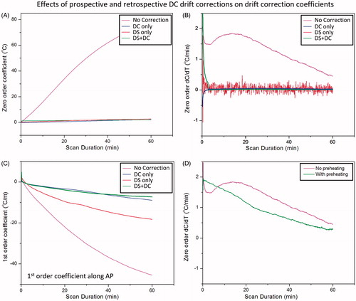
Figure 7. Correction of phase-induced image shift using F0 dynamic stabilisation (DS). In the absence of DS, there is a gradual shift in image position along the phase encoding direction over time, corresponding to approximately 1 mm after 15 min of scanning (upper curve, red). A negative shift (<0.5 mm after 30-min scan) is observed along the frequency encoding direction (lower curve, pink). Both image shifts are corrected after applying DS (middle curves, blue and green). Right panel are corresponding magnitude maps showing the position shift over time with DS turned on/off.
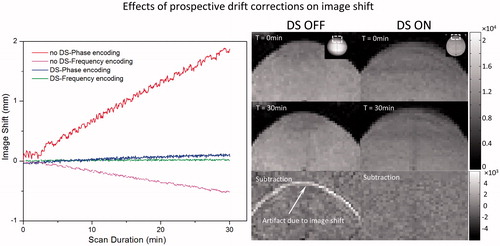
Figure 8. Comparison is made between fibre-optic measurements and MR thermometry using various drift correction strategies: raw data (No Correction) dynamic stabilisation only (DS), DC+ 3D drift correction algorithm only (DC+ 3D), and combined strategy (DS and DC+ 3D). The drift correction algorithm validated here is the combination of DC drift correction and 3D first order drift correction. Panels A and B represent data acquired at probe 1 and probe 2 (shown in the insert), representing the heated and unheated region, respectively.
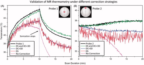
Table 2. Influence of F0 dynamic stabilisation and different kinds of retrospective drift correction algorithm on the accuracy of temperature measurements with PRF-shift MR thermometry in a gellan gum phantom.
Table 3. MR temperature measurements acquired in 16 rabbits treated with MR-HIFU hyperthermia. MR temperature mapping used both prospective and retrospective corrections, with pre-heating and F0 dynamic stabilisation, and combined drift correction algorithm. Temperature is well maintained at 41–45 °C in treatment cells for the intended duration (Time in Range). During therapy, mean temperature in treatment cells is 42.3° ± 0.7 °C, with T10 and T90 of 43.3° ± 0.8 °C and 41.4° ± 0.7 °C. The rectum temperature is not affected by treatment (37.1° ± 0.3 °C, with a temporal SD of 0.3° ± 0.2 °C).
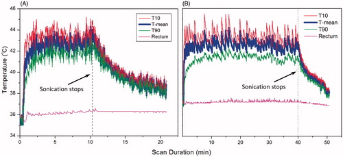
Figure 9. Temperature measured in a target region of rabbit muscle with MR thermometry during (A) 10 and (B) 40 min of hyperthermia. MR temperature maps were calculated from EPI acquisition, with pre-heating, F0 dynamic stabilisation, and combined drift correction algorithm. The mean (T-mean, thick blue curve), T10, thin red upper curve (90th percentile) and T90, thin green lower curve (10th percentile) are shown in the graph. The temperature of the animal’s rectum during the treatment is plotted in the pink flat curve around 36-37 degree. The graphs indicate localised and well controlled heating in the target region with minimal heating of distal areas.