Compact self-grounded Bow-Tie antenna design for an UWB phased-array hyperthermia applicator

Figures & data

Figure 1. (a) The model of the self-grounded Bow-Tie antenna. (b) Schematic drawing of the manufactured antenna with its dimensions indicated, top and side views.

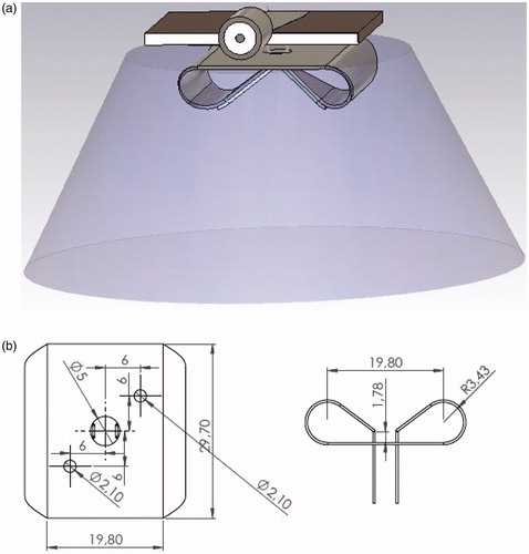
Figure 2. Tapered balun geometry (a) front side and (b) back side.

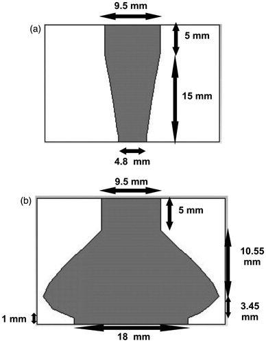
Figure 3. Visualisation of the muscle load configuration.

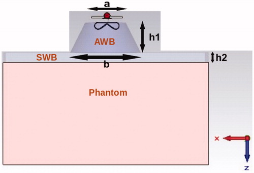
Figure 4. Setup for evaluation of penetration coefficient, p_fTS.

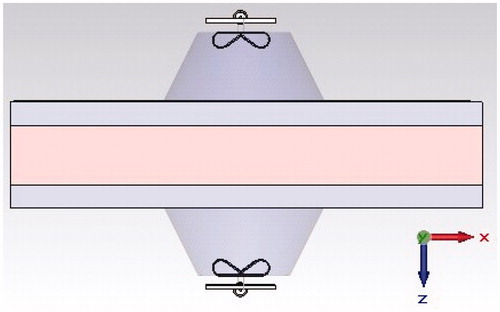
Figure 5. (a) Back-to-back balun and (b) simulated reflection and transmission coefficients of the balun in back-to-back configuration.

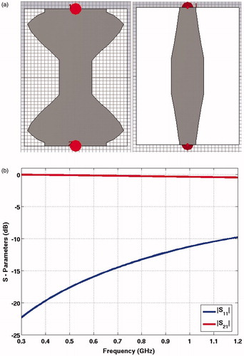
Figure 6. Variation of the reflection coefficient of the antenna for various pin widths (simulated).

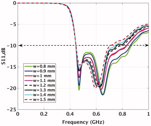
Figure 7. The effect of dielectric layers with 7.7 mm length on surface current density of the antenna at 500 MHz. (a) No dielectric and (b) dielectrics.

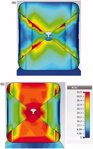
Figure 8. The effect of permittivity of dielectric layer on reflection coefficients of the antenna.

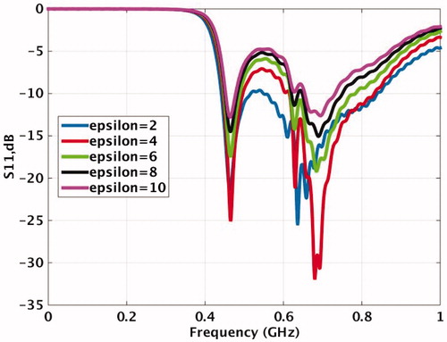
Figure 9. The effect of dielectric layers on E-field of the antenna at frequency 430 and 700 MHz along the cross section of the antenna at y = 0. E-fields are in V/m.

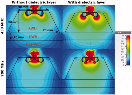
Figure 10. Impact of dielectric layers on reflection coefficient of antenna immersed in large and limited AWB. The red and blue curves show the S₁₁ without and with Teflon in conical shape AWB, respectively. The black and green curves show the S₁₁ without and with Teflon in rectangular shape AWB, respectively.

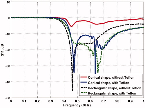
Figure 11. Impact of length of dielectric layer on reflection coefficient of the antenna.

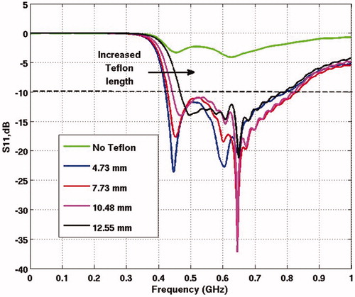
Figure 12. The power loss density distribution in the muscle phantom for different AWB shapes. (a) Rectangular AWB without dielectric layer on the antenna arms. (b) Rectangular AWB with dielectric layer. (c) Cylindrical AWB. (d) Conical AWB.

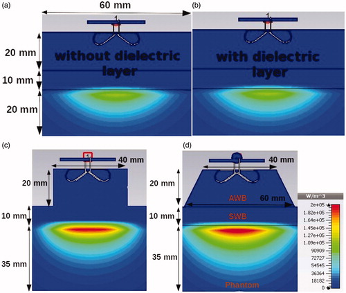
Figure 13. The reflection coefficient of the antenna with three different shapes of AWB.

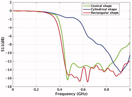
Figure 14. Dependence of the EFS on dimensions of the water bolus.

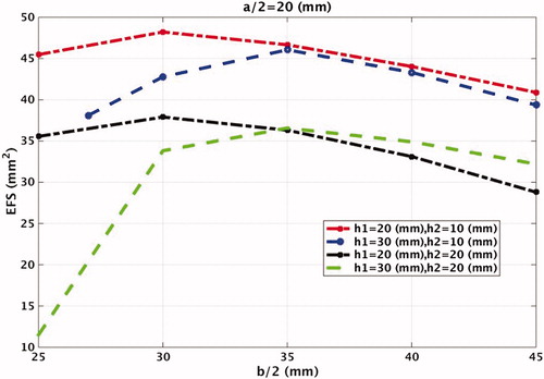
Figure 15. Dependence of the RC_BW on dimensions of the water bolus.

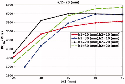
Table 1. p_fTS in terms of AWB dimensions.

a/2, b/2, h1,h2 (mm)	pfTS (dB)
20,30,30,10	−9.0976
20,35,20,10	−9.3832
20,30,30,10	−3.8653
20,35,30,10	−8.0304
20,30,20,20	−9.9712
20,35,20,20	−9.9633
20,30,30,20	−9.4001
20,35,30,20	−8.8897

Figure 16. Sensitivity of the reflection coefficient to temperature variations in water bolus.

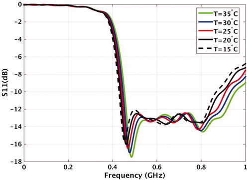
Figure 17. Simulated power loss density distribution in muscle phantom for various frequencies. (a) 430 MHz, (b) 500 MHz, (c) 600 MHz, (d) 700 MHz and (e) 900 MHz.

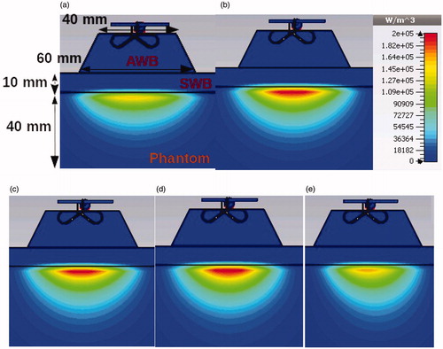
Figure 18. The prototype of the manufactured antenna, including the UWB balun and the plastic enclosure.

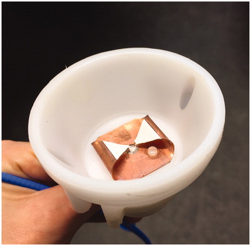
Figure 19. Measured and simulated reflection and transmission coefficients of the antenna.

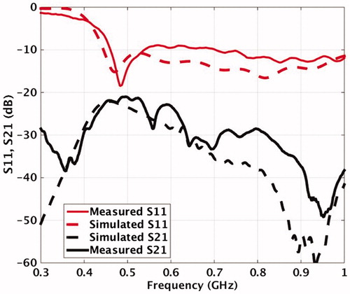
Figure 20. (a) The temperature rise distribution in a muscle phantom after exposure of 10 W for 9 min. (b) The SAR distribution in muscle phantom calculated from the measured temperature distribution. (c) The simulated SAR distribution in the muscle phantom. Frequency was 500 MHz in all cases.

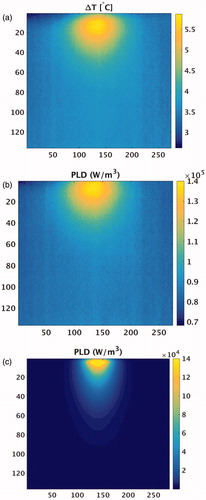
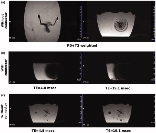
Figure 21. The magnitude of MR images (a) proton density + T2-weighted images in middle-coronal and axial plane, without connector. (b) The echo time images in the axial plane, with connector. (c) The echo time images in the axial plane, without connector.