
Figures & data
Figure 1. Schematic diagram of the AMC-2 system. The dorsal or bottom antenna is integrated in the table. The ventral or top antenna and bolus are mounted on a lift. The antennas are connected via a tuner to a phase- and amplitude-controlled generator. The temperature-controlled demineralised water in each bolus can be cooled or heated depending of the depth of the tumour (top diagram). The blue arrows indicate the movement options of the antennas (bottom diagram). Both antennas can be rotated 180° for flexible positioning.
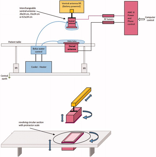
Figure 2. Left: the three waveguide sizes, left to right the 20 × 34, 15 × 34 and 8.5 × 34 cm waveguide. Right: schematic drawing of the 15 × 34 cm applicator with conductor rod. The distances between rod and aperture and between the rod and the back plate of the waveguide are 93 and 36.5 mm, respectively.
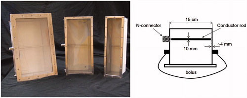
Figure 3. Schematic drawing of the experimental set-up for the E-field measurements. Top left: the elliptical phantom, the interchangeable applicator and at the bottom side the 20 × 34 cm applicator. Bottom right: the sagittal YZ and transversal XY measurement planes.
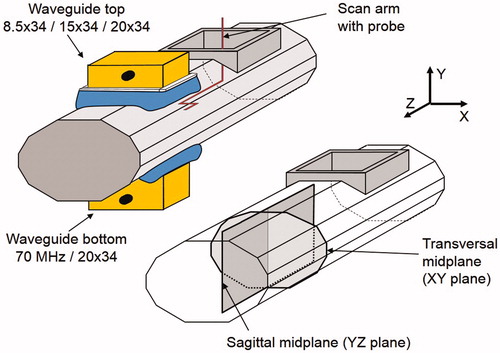
Table 1. Overview of all E-field measurements.
Figure 4. Clinical set up for a 72-year-old male patient with a 10 × 10 cm melanoma located in the left axilla. The 8.5 × 34 cm waveguide was applied as ventral antenna at the top. The 20 × 34 cm applicator was located at the dorsal side. A 1.67 mm (5F) thermometry catheter was placed invasively over a length of 10 cm in the tumour.
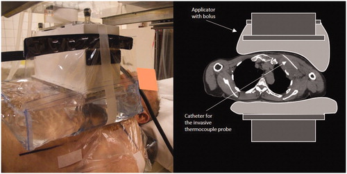
Figure 5. Contour plots of the E-field (Z-component) of the 20 × 34, 15 × 34 and 8.5 × 34 cm antennas (from left to right). The top row shows the distributions in the central transversal XY-plane and the bottom row the distributions in the sagittal YZ-plane (). The Z-component of the E-field in the centre of the phantom was normalised to 100%.
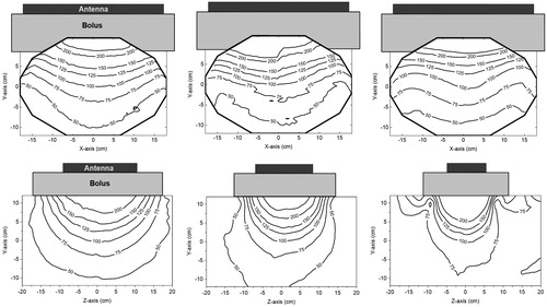
Figure 6. E-field distributions of the different antenna combinations at zero phase. From left to right: The contour plots of the 20 × 34 + 20 × 34 cm, 20 × 34 + 15 × 34 cm and 20 × 34 + 8.5 × 34 cm antenna combinations. The first row shows the field distributions in the transversal XY-plane and on the second row shows the distributions in the sagittal YZ-plane (). The Z-component of the E-field in the centre of the phantom was normalised to 100%.
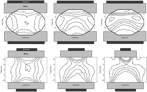
Table 2. FWHM, i.e. the width where the SAR is 50% of maximum SAR, determined at the centre of the phantom and at 4 cm below the top antenna.
Figure 7. E-field profiles measured along the central transversal Y-axis of the phantom for different two-antenna set-ups. Measurements were performed for seven different phase settings of the bottom antenna: 120°, 90°, 45°, 0, −45°, −90° and −120° for the 20 × 34 + 20 × 34 cm (top graph), the 20 × 34 + 15 × 34 cm (central graph) and the 20 × 34 + 8.5 × 34 cm antenna combination (bottom graph). All graphs are a fit (sixth degree polynomial) to the measured data. The E-field was normalised in the centre of the phantom at zero degrees phase difference.
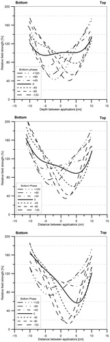
Figure 8. Contour plots of the field distribution in the transversal mid-plane for a symmetrical (top) and an asymmetrical (bottom) set-up using the 20 × 34 + 15 × 34 cm antenna combination with a −120° phase for the bottom antenna. In the asymmetrical set-up, the phantom was shifted 10 cm to the left. The Z-component of the E-field in the centre of the phantom was normalised to 100% at zero phase.
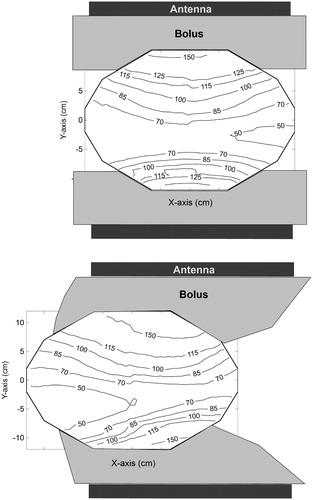
Figure 9. SAR profiles as function of the depth on the central transversal axis of the elliptical phantom, for the three different applicators (20 × 34, 15 × 34 and 8.5 × 34 cm).
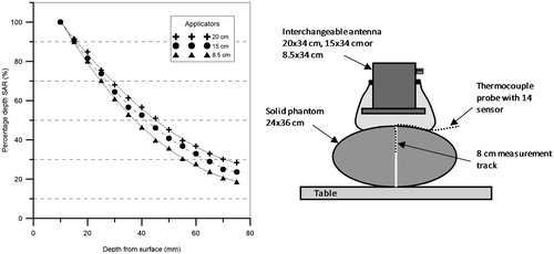
Figure 10. Measured reflection loss (S11) as function of frequency for the three waveguides (20 × 34, 15 × 34 and 8.5 × 34 cm). All waveguides are positioned on top of the phantom with a 6 cm bolus in the left graph, and positioned on the chest of a volunteer with ∼6 cm upper bolus in the right graph.
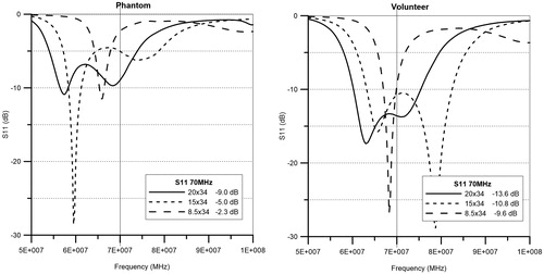
Table 3. Measured values of the reflection coefficient (S11), VSWR and the relative reflected power for each antenna positioned on an elliptical saline phantom with a bolus of 6 cm between antenna and phantom.
Figure 11. Simulated E-field distributions and profiles of the 20 × 34 + 20 × 34 antenna combination. The distribution in the transversal XY-plane (left), the distribution in the sagittal YZ-plane (middle) and the E-field profiles on the central Y-axis for seven different phase settings (120°, 90°, 45°, 0, −45°, −90° and −120°) of the bottom antenna with respect to the top antenna (right). The Z-component of the E-field in the centre of the phantom was normalised to 100% at 0° phase difference.
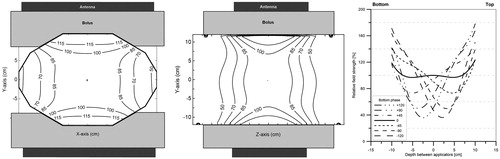
Table 4. Treatment results for a male patient with a melanoma in the left axilla.