Figures & data
Figure 1. Flowchart of our methodology for computation of the ultimate SAF. STEP #1: The electric and magnetic dipoles in the dipole cloud are excited using random amplitudes and phases. STEP #2: The incident electric fields created by these excitations are computed using the analytical free-space Green’s function at the treatment frequency. STEP #3: Total electric fields are computed using the fast volume integral equation solver MARIE. Steps #1–#3 are repeated as many times as there are fields in the basis-set (2500 times in our case). STEP #4: The combination weights x applied to the basis fields are optimised so as to maximise the SAF in the target tumour volume. STEP #5: The SAR map associated with the SAF of STEP #4 is computed by applying the weights x to the basis fields. STEP #6: The temperature map is then computed by solving the Pennes bio-heat equation using the SAR map of STEP #5 as a source term. The input power of the SAR map is scaled so as to reach a maximum temperature of 45 degrees after 30 min of hyperthermia treatment. STEP #7: The thermal dose is computed by applying the CEM43 formula to the temperature histories computed in STEP #6.
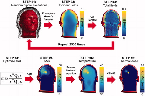
Figure 2. A: Conductivity map in the transverse view overlaid with the modelled tumour locations #1–#8. B: Convergence of SAR amplification factors (SAF) as a function of the number of basis fields in the basis-set for eight of the twelve tumour locations (F = 127.7 MHz). C: Conductivity map in the sagittal view overlaid with the last four tumour locations. D: Convergence of the SAF as a function of the number of basis fields for tumour #9 (F = 127.7 MHz). The purple curve corresponds to the original tumour #9 in direct contact with air. The black curve corresponds to a modified version of tumour #9 in which a 1-voxel thick layer of skin was added between the tumour and air. The two numbers above these curves indicate the percent change of SAF per additional 1000 basis field. E: Convergence of SAFs at F = 127.7 MHz as a function of the number of fields for tumour locations #10, #11 and #12.
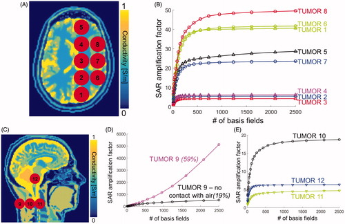
Table 1. Simulations and metrics of this study.
Figure 3. USAFs as a function of the HT treatment frequency for tumours #1 through #12. The red numbers indicates, for each tumour location, the ratio of the highest to the lowest uSAF. In other words, this ratio indicates the expected improvement in SAF treatment efficacy by optimising the treatment frequency.
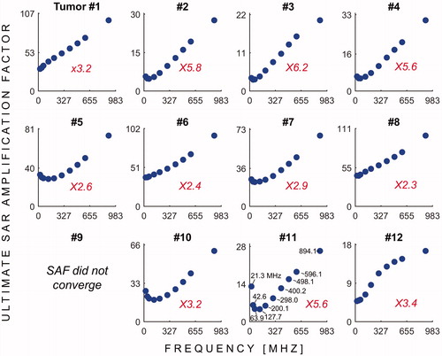
Figure 4. USAFs (log scale) as a function tumour depth for all the frequencies simulated. The red numbers and solid blue dots indicate the uSAFs for the shallowest and deepest tumour locations at each frequency.
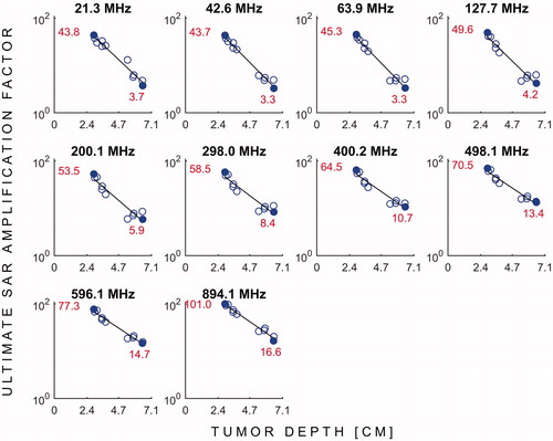
Figure 5. SAR maps (in W/kg) associated to the uSAF HT treatment for tumours #3–#6 at frequencies 127.7, 400.2, 596.1 and 894.1 MHz in both the transverse and sagittal views. Contours of the head and the tumour are shown in green. The white numbers indicate the uSAF for each tumour location and frequency simulated. USAFs are computed for the whole head and are, therefore, the same for the transverse and sagittal views.
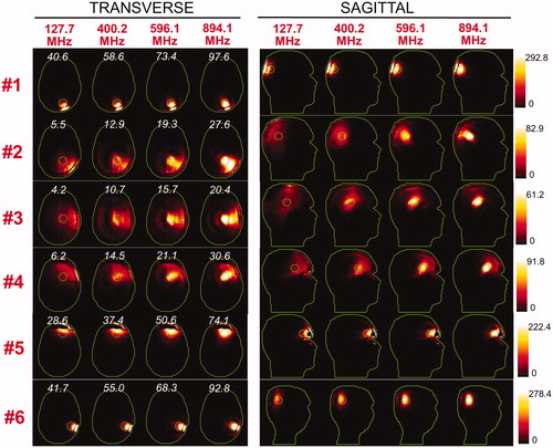
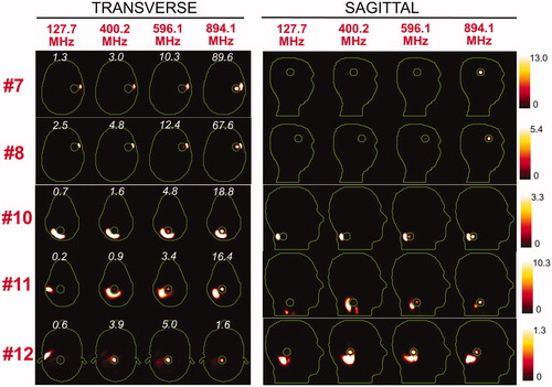
Figure 6. SAR maps (in W/kg) associated to the uSAF treatment for tumours #7–#12 at frequencies 127.7, 400.2, 596.1 and 894.1 MHz in both the transverse and sagittal views. Tumour #9 is not shown since the SAF did not converge to the ultimate value for this tumour location. Contours of the head and the tumour are shown in green. The white numbers indicate the uSAF for each tumour location and frequency simulated. USAFs are computed for the whole head and are, therefore, the same for the transverse and sagittal views.
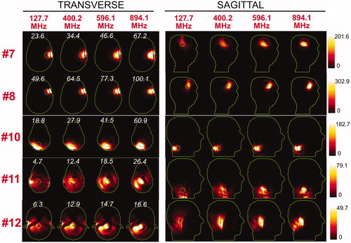
Figure 7. Temperature maps associated with the uSAF HT treatment for tumours #3–#6 and frequencies 127.7, 400.2, 596.1 and 894.1 MHz. The slices shown are transverse and sagittal views of the temperature volume though the centre of the tumours. Input SAR maps are scaled so as to achieve a maximum temperature of 45 degrees at the end of the 30-min HT treatment. Note that the maximum temperature is not necessarily achieved inside the tumour. Contours of the head and the target tumour ROI are shown in green. The white numbers indicate the temperature amplification ratio, which is the ratio of the average temperature increase inside and outside the tumour. Temperature amplification ratios are computed for the whole head and are, therefore, the same for the transverse and sagittal views.
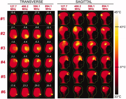
Figure 8. Temperature maps associated with the uSAF HT treatment for tumours #7–#12 and frequencies 127.7, 400.2, 596.1 and 894.1 MHz. Tumour #9 is not shown since the SAF did not converge to the ultimate value for this tumour location. The slices shown are transverse and sagittal views of the temperature volume though the centre of the tumours. Input SAR maps are scaled so as to achieve a maximum temperature of 45 degrees at the end of the 30-min HT treatment. Note that the maximum temperature is not necessarily achieved inside the tumour. Contours of the head and the target tumour ROI are shown in green. The white numbers indicate the temperature amplification ratio, which is defined as the ratio of the average temperature increase inside and outside the tumour. Temperature amplification ratios are computed for the whole head and are, therefore, the same for the transverse and sagittal views.
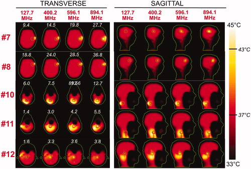
Figure 9. Maps of the cumulative equivalent minute at 43 degrees (CEM43) thermal dose for tumours #1–#6, computed from the temperature histories of Figure 7. The white numbers indicate the thermal dose amplification ratio, which is the ratio of the average thermal dose inside and outside the tumour, for every tumour location and frequency. Thermal dose amplification ratios are computed for the whole head and are, therefore, the same for the transverse and sagittal views.
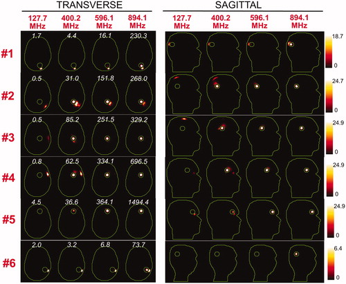
Figure 10. Maps of the cumulative equivalent minute at 43 degrees (CEM43) thermal dose for tumours #7–#12, computed from the temperature histories of Figure 7. Tumour #9 is not shown since the SAF did not converge to the ultimate value for this tumour location. The white numbers indicate the thermal dose amplification ratio, which is defined as the ratio of the average thermal dose inside and outside the tumour, for every tumour location and frequency. Thermal dose amplification ratios are computed for the whole head and are, therefore, the same for the transverse and sagittal views.