Commentary on the clinical and preclinical dosage limits of interstitially administered magnetic fluids for therapeutic hyperthermia based on current practice and efficacy models

Figures & data

Table 1. Exemplar guidelines for the maximum injection volumes of experimental compounds in mice, rats, rabbits and humans (of the given FDA reference body weights) on the basis of the administration route, as used by the Duke University Medical Center in Durham, NC, USA [47].

Route	Mouse (20 g)	Rat (150 g)	Rabbit (1.8 kg)	Human (60 kg)
Subcutaneous	2 ml/site	10 ml/site	50 ml/site	2 ml/site
Intramuscular	0.1 ml/site	0.3 ml/site	0.5 ml/site	5 ml/site
Intraperitoneal	3 ml	10 ml	100 ml	5 ml
Intravenous	0.2 ml	0.5 ml	5 ml	250 ml
Intradermal	0.05 ml/site	0.05 ml/site	0.1 ml/site	0.1 ml/site

Figure 1. Equilibrium temperature profile ΔT(r) within and surrounding a sphere of radius R of a medium of thermal conductivity within a medium of thermal conductivity , after prolonged exposure to an energy source depositing power P into the sphere [74]. The solid lines represent solutions to Equation (8)(8a) for values of the ratio / ranging from 1.0 to 2.0, plotted in the reduced coordinate system where r′ = r/R, and ΔT′(r′) = 3 ΔT(r)/PR².

Figure 2. Illustrative bioheat model calculations in the steady-state, zero perfusion, zero metabolic heat generation limit, for a 60 kg human, as per Equation (10)(9) , showing ΔT_R isotherms in the V_i-c plane, where ΔT_R is the equilibrium temperature at the surface of a sphere of radius R containing a uniform distribution of heat-evolving magnetic nanoparticles. Assumed parameters are: intrinsic loss power ILP = 3.0 nHm²/kg_Fe; dispersion factor v = V_d/V_i = 2.4; thermal conductivity of the surrounding medium λ₂ = 0.52 W/Km; and activation field amplitude H = 5 kA/m and frequency f = 300 kHz. The shaded region demarcates the clinically acceptable dose region, as determined from both the material loading capacities of the local tissue, viz. 40 mg_Fe/ml_tissue, and of the body as a whole, viz. 850 mg_Fe. The latter value is derived, as per Equation (6)(6) , assuming a “good” agent formulation scenario of relatively high retention ( = 0.85) and systemic tolerance ( = 0.85). The points A and B denote two possible treatment scenarios, as discussed in the text.

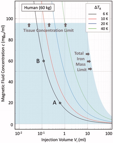
Figure 3. Illustrative bioheat model calculations in the steady-state, zero perfusion, zero metabolic heat generation limit, for a 20 g mouse, as per Equation (10)(9) , under the same material conditions as in Figure 2, viz. ILP = 3.0 nHm²/kg_Fe, v = V_d/V_i = 2.4, and λ₂ = 0.52 W/Km. The solid lines are ΔT_R = 6 K isotherms, indicating the thresholds for therapeutic hyperthermia. The shaded region demarcates the murine “acceptable dose region”, as determined from both the material loading capacities of the local tissue, viz. 40 mg_Fe/ml_tissue, and of the mouse as a whole, viz. 3.5 mg_Fe. The latter value is derived, as per Equation (6)(6) , assuming a “good” agent formulation scenario of relatively high retention ( = 0.85) and systemic tolerance ( = 0.85). The red line, corresponding to H = 5 kA/m and f = 300 kHz (the same conditions as in Figure 2), lies outside the acceptable dose region, and as such is inaccessible. The black line, corresponding to H = 10 kA/m and f = 1 MHz, lies within the acceptable dose region, as therefore is accessible. The points A, A′, B and B′ are discussed in the text.

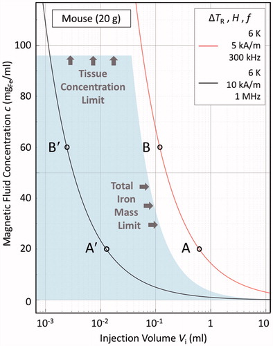
Figure 4. Comparison between maximum temperature rises ΔT_max due to magnetic heating as calculated using the first-order approximation method of Equation (8)(8a) and (10)(9) , and the reported ΔT_max for a clinical study of prostate cancer patients undertaken by the MagForce team [61]. The limitations of the zero-perfusion, zero-metabolism model are evident at the lower ΔT_max values, but the model is more valid as ΔT_max increases. The arrow denotes the ΔT_max value for which the temperature of the entire magnetic-nanoparticle-infused tissue volume reaches the therapeutically significant value of ΔT = 6 K or above. The dashed line is a guide to the eye only.

Nair AB, Jacob S. (2016). A simple practice guide for dose conversion between animals and human. J Basic Clin Pharm 7:27–31.

 PubMedGoogle Scholar

Andrä W, d’Ambly C, Hergt R, et al. (1999). Temperature distribution as function of time around a small spherical heat source of local magnetic hyperthermia. J Magn Magn Mater 194:197–203.

 Web of Science ®Google Scholar

Johannsen M, Gneveckow U, Thiesen B, et al. (2007). Thermotherapy of prostate cancer using magnetic nanoparticles: feasibility, imaging, and three-dimensional temperature distribution. Eur Urology 52:1653–61.

 PubMed Web of Science ®Google Scholar