Figures & data
Figure 1. Antenna blueprint with distances in millimetre. Distance (d) and water temperature (T) are varied in the experiments. Distance (d) is varied by changing the distance that the antenna protrudes into the water-filled container (purple region).
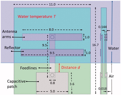
Table 1. Design specifications and constraints for the development of the antenna.
Figure 2. Applicator with embedded antenna, water bolus and animal placeholder in Experiment 1. Note that the animal mimicking phantom in Experiment 2 was positioned 4 mm lower and had a 20 mm diameter. The black dots in the left picture mark temperature sensor locations.
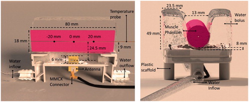
Table 2. The material properties used in the electromagnetic and heat flow models.
Figure 3. (a) Reflection coefficient for various water levels as measured at a water temperature of 37 °C. (b) Reflection coefficient for various water temperatures at a distance (d) of 3.0 mm.
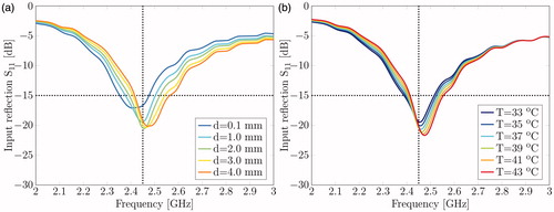
Figure 4. The temperature profiles as generated from heating a cylindrical phantom with 16.5 W effective power at three locations: the middle and 2 cm shifted in each direction along the longitudinal axis. Measured (solid lines) and simulated (dashed lines) time–temperature profiles.
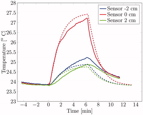
Figure 5. Simulated (a) and measured (b) temperature distributions (°C) for Experiment 2 (phantom length 80 mm, diameter 20 mm).
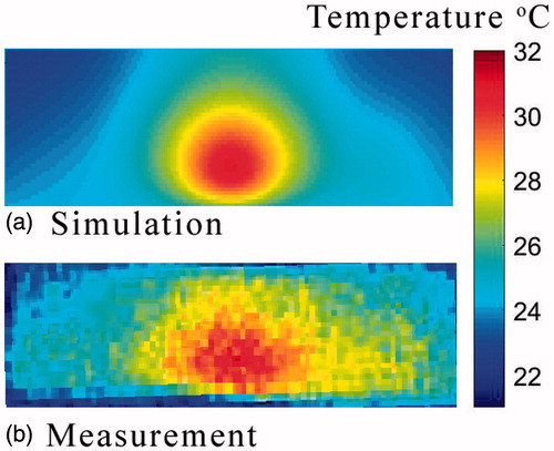
Figure 6. Magnitude scan of the applicator. The antenna is located in the red square at the lower centre region.
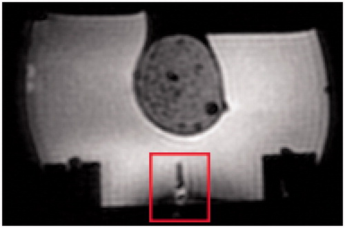
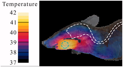
Figure 7. A cutout of the temperature distribution in Celcius degrees as generated by the antenna radiating at 20 W. The boundary of the sensitive tissues is marked by the white dashed line and the target area with cyan.