Feasibility of on-line temperature-based hyperthermia treatment planning to improve tumour temperatures during locoregional hyperthermia

Figures & data

Figure 1. Transversal cross-sections of the CT scan for the three patients. The contour indicates the target region. Cross-sections are at the centre of the target region in axial direction.

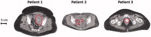
Figure 2. Photograph of the 70 MHz AMC-8 system (left) and a schematic picture of a patient in a single ring four-antenna set-up (right).

Table 1. Values of the tissue properties used in the simulations; conductivity (σ [S m⁻¹]), relative permittivity (ε_r [–]), density (ρ [kg m⁻³]), specific heat capacity (c [J kg⁻¹ °C⁻¹]), thermal conductivity (k [W m⁻¹ °C⁻¹]) and perfusion (w_b [kg m⁻³s⁻¹]).

	σ (S m^−1)	εr (–)	ρ (kg m^−3)	c (J kg^−1 °C^−1)	k (W m^−1 °C^−1)	Wb (kg m^−3 s^−1)
Air	0	1	1.29	10 000*	0.024	0
Bone	0.05	10	1595	1420	0.65	0.12
Fatty	0.06	10	888	2387	0.22	1.1
Lung	0.2	20	750	3000	0.25	3.6
Muscle-like	0.75	75	1050	3639	0.56	3.6
Tumour	0.74	65	1050	3639	0.56	1.8

* The value of c used for air was 10 times too high in order to allow larger time steps in thermal computations. This has a negligible effect on the steady state temperature.

Figure 3. Screenshot of the graphical user interface for on-line use of hyperthermia treatment planning. Phase-amplitude settings can be adapted on the left hand-side. The corresponding predicted temperature distribution is instantly projected onto the CT scan. In the top right window the temperature volume histogram of the delineated target region is shown, with a summary of the indexed temperatures T₁₀, T₅₀ and T₉₀ and minimum and maximum temperature.

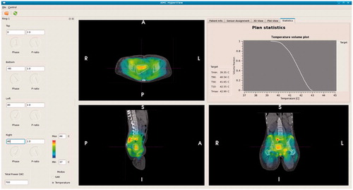
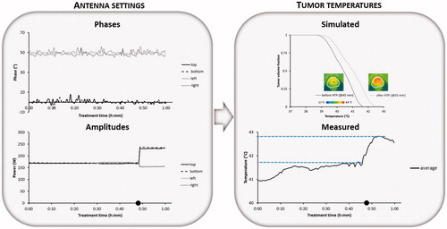
Figure 4. Example showing phase-amplitude steering for patient 1 (pelvic melanoma metastasis) with recorded phases and amplitudes per antenna, the average measured temperature during the steady state period and the simulated temperature distribution in the tumour with the simulated temperature volume histogram before and after adaptation of the phase-amplitude settings based on treatment planning. Symbol • indicates the time at which phase-amplitude steering was performed to improve tumour temperatures.

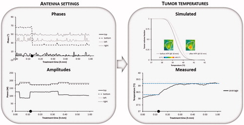
Figure 5. Example showing phase steering for patient 2 (cervix) with recorded phases and amplitudes per antenna, the average measured temperature during the steady state period and the simulated temperature distribution in the tumour with the simulated temperature volume histogram before and after adaptation of the phases based on treatment planning. Symbols • indicate the times at which phase steering was performed to improve tumour temperatures.

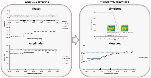
Figure 6. Example showing amplitude steering for patient 3 (cervix) with recorded phases and amplitudes per antenna, the average measured temperature during the steady state period and the simulated temperature distribution in the tumour with the simulated temperature volume histogram before and after correction of the amplitude settings based on treatment planning. Symbol • indicates the time at which amplitude steering was performed to improve tumour temperatures.