Real-time 3D ultrasound based motion tracking for the treatment of mobile organs with MR-guided high-intensity focused ultrasound

Figures & data

Figure 1. 3 D ultrasound (US)-based motion tracking and MR-thermometry pipeline. Schematic of the 3D US-based motion estimation system. The 256 elements HIFU transducer is represented in grey. Transducer elements operating in emission are represented in green and those in reception in blue, respectively. ($\overrightarrow{\mathrm{x}},\overrightarrow{\mathrm{y}},\overrightarrow{\mathrm{z}})$ is the transducer spatial reference frame of coordinates, where the displacement $\overrightarrow{\mathrm{D}}$ (green arrow) is estimated. $\overrightarrow{{\mathrm{a}}_{\mathrm{i}}\mathrm{ }},\mathrm{ }\mathrm{i}\in \left[\mathrm{1,4}\right]$ represents the normal vector of each sub-aperture along which the displacement is measured using a pulse-echo mode. The pipeline of 3D displacement estimation is presented underneath. TOF: Time Of Flight for US to reach the depth of interest; motion correction (MOCO): computing time for the displacement estimation, UPDATE: transducer phase law update (see Methods section for details). HIFU: additional US sonication to induce temperature increase of the tissue. Refresh rate is given by durations of TOF (150 µs for typical distance of 12 cm) + MOCO (18 ms) + UPDATE (19 ms) + HIFU (adjustable depending on desired update rate). (Colored version is available on the journal’s webpage).

Figure 2. Displacement estimation pipeline.1. Ultrasound (US) signal acquisition was performed at 100 MHz and 1400 samples were acquired. The first acquisition (t = 0) was taken as the reference (US signals surrounded in red).2. Decision tree: Absolute displacement (reset to initial position${FP}_t=\left[0 0 0\right]$) was made if normalised cross-correlation of the current and reference data ($\overline{{\mathrm{C}\mathrm{o}\mathrm{r}\mathrm{r}}_{\mathrm{t}=0,\mathrm{t}+\mathrm{d}\mathrm{t}}}$) was greater than a predefined threshold (0.998 in vitro and 0.98 in vivo). If normalised cross-correlation ($\overline{{\mathrm{C}\mathrm{o}\mathrm{r}\mathrm{r}}_{\mathrm{t},\mathrm{t}+\mathrm{d}\mathrm{t}}}$) was greater than 0.8, a relative displacement between t and t + dt was performed, and data were discarded otherwise.3. Computation of normalised cross-correlations and extraction of temporal lags T_i.4. Computation of the displacement $\overrightarrow{D}$ in ($\overrightarrow{\mathrm{x}},\overrightarrow{\mathrm{y}},\overrightarrow{\mathrm{z}})$ by solving a pseudo-inverse problem [see Equation (1)(1) $$T_i=\frac{2}{c}.A.D\mathrm{ }i\in \left[1:4\right]$$(1) ].5. Update of the current focus position ${FP}_{t+dt}\text{.}$(Colored version is available on the journal’s webpage).

Figure 3. In vitro and in vivo validation. (a) The rotation of a motor is converted into a 1D translation along y-axis, using a rod and slides. The phantom is maintained above the transducer using a plastic box with a Mylar membrane glued at the bottom to allow propagation of the ultrasound beam. Typical motion settings were 10 mm of amplitudes and maximum velocities of 10 mm.s⁻¹. Three coronal slices were acquired to monitor MR-thermometry. (b) Transverse ((x, z) plane in the transducer’s frame of reference) anatomical image of the setup. Blue box represent three slices in coronal orientation and green box represent the crossed pair navigator position. (c) Anatomical image and animal positioning. Blue box represent five MR-temperature slices positioned in coronal orientation. A saturation slab (yellow box) was positioned on top of the hepatic dome to suppress signal from the heart on the images. (d) Diagram of sonication locations in pig #2 (L1–L3), blue circles depict the focus locations for each ablation. Note that for each location a reference sonication was performed at the same location without focus position correction. Sonication locations in pig #1 (2 locations separated by 1 cm) were performed in the same anatomical region of the liver (data not shown). (Colored version is available on the journal’s webpage).

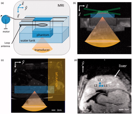
Figure 4. Displacement estimation validation in vitro. (a) MR-navigator signal positioned along the y-axis acquired during 21 s. (b) Representative displacement estimations in ($\overrightarrow{\mathrm{x}},\overrightarrow{\mathrm{y}},\overrightarrow{\mathrm{z}})$ obtained in vitro using our experimental settings. The blue and green curves represent the displacement estimations and the corresponding instantaneous speed computed from estimated positions, respectively. The bottom graph displays the normalised cross-correlations between two successive US acquisitions along time, for each sub-apertures. Black arrows depict lower normalised cross-correlation coefficients during peak velocities. On the bottom graph, the red curve represents the mean correlation between current measurement and the first acquisition taken as reference. The black dashed line represents the threshold above which absolute displacement estimations is performed to reset the position. (Colored version is available on the journal’s webpage).

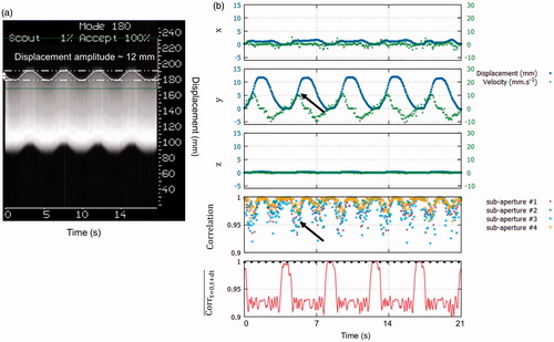
Figure 5. Representative in vitro MR-thermometry. (a) Shows temperature images overlaid to magnitude images, taken at the end of HIFU sonication, without (top) and with (bottom) 3D focus position update. (b) Shows the temperature temporal evolution of the pixel experiencing the maximum temperature increase, for both conditions. The 50 first dynamic acquisitions (grey box) corresponded to the learning step in the thermometry pipeline and were used for correction of motion and associated susceptibility artefacts of temperature images. (c) shows the temperature profiles along the y-axis crossing the pixel with maximal temperature increase, at the end of sonication, for both conditions. (Colored version is available on the journal’s webpage).

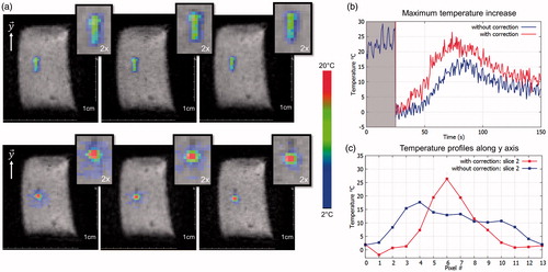
Table 1. Summary of the five ablations performed on gel phantom.

		Duration of sonication (s)	Acoustic power (W)	Displacement amplitude on y-axis (mm)			Maximum temperature (°C)		FWHM [X × Y] (mm × mm)
				Before sonication	During sonication	After sonication	Without correction	With correction	Without correction	With correction
L1	#1	30	150	12 ± 1	11 ± 1	12 ± 1	18	25	6 × 18	6 × 6
	#2	30	150	12 ± 1	12 ± 1	11 ± 1	18	26	6 × 18	5 × 6
L2	#3	30	150	10 ± 2	10 ± 1	11 ± 1	17	22	7 × 17	6 × 7
	#4	30	150	10 ± 1	10 ± 1	9 ± 2	17	23	7 × 17	5 × 7
L3	#5	30	150	11 ± 1	10 ± 1	10 ± 1	19	26	8 × 16	6 × 6

This table reports the ultrasound power, the sonication duration, the displacement estimations before/during/after sonication on y-axis, the maximum temperature increase without and with focus position correction and finally the resulting FWHM of temperature images without and with focus position correction, respectively.

Figure 6. Displacement estimation in vivo in pig liver. (a) MR-navigator signal positioned along the y-axis acquired during 30 s. (b) Representative displacement estimations in ($\overrightarrow{\mathrm{x}},\overrightarrow{\mathrm{y}},\overrightarrow{\mathrm{z}})$ obtained during in vivo experiment on liver. The blue and green curves represent the displacement estimations and the corresponding instantaneous speed computed from estimated positions, respectively. The bottom graph displays the normalised cross-correlations between two successive US acquisitions along time, for each sub-apertures. The red curve displays the mean correlation between current and the first acquisition taken as reference. The black dashed line represents the threshold above which absolute displacement estimations is performed to reset the position. (Colored version is available on the journal’s webpage).

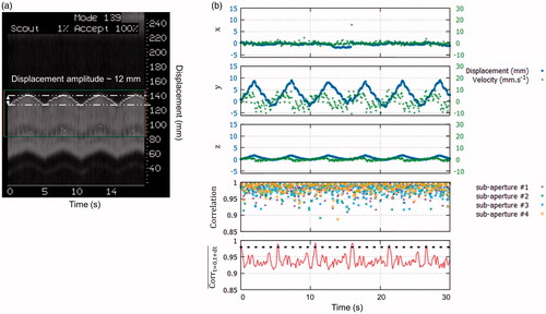
Figure 7. Representative in vivo MR-thermometry. (a) Screen capture of representative temperature images overlaid to magnitude image, taken at the end of HIFU sonication, without (top) and with (bottom) focus update. (b) Shows the temperature evolution of the pixel experiencing the maximum temperature increase, along time, for both conditions. The 50 first dynamic acquisitions (grey box) corresponded to the learning step in the thermometry pipeline (see Methods for details). (c) shows the temperature profile along the axis crossing the pixel with maximal temperature increase at the end of sonication, for both conditions. (Colored version is available on the journal’s webpage).

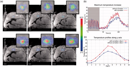
Table 2. Summary of the eight ablations performed in the liver of pigs.

		Duration of sonication (s)	Acoustic power (W)	Displacement amplitude on y-axis (mm)			Maximum temperature (°C)		FWHM [X × Y] (mm × mm)
				Before sonication	During sonication	After sonication	Without correction	With correction	Without correction	With correction
L1	#1	10	325	8 ± 1	9 ± 1	9 ± 2	8	10	7 × 9	6 × 7
	#2	10	325	9 ± 2	8 ± 1	9 ± 1	7	9	8 × 11	8 × 8
	#3	15	325	9 ± 1	9 ± 2	NA	10	13	7 × 11	8 × 7
	#4	20	560	9 ± 1	9 ± 1	11 ± 4	10	14	6 × 7	6 × 4
L2	#5	40	560	9 ± 2	10 ± 1	9 ± 3	18	27	12 × 13	8 × 9
L3	#6	40	560	10 ± 1	10 ± 1	9 ± 1	20	26	8 × 12	7 × 8
L4	#7	40	560	8 ± 1	9 ± 1	9 ± 1	18	24	10 × 13	8 × 8
L5	#8	40	560	9 ± 2	10 ± 1	9 ± 1	17	25	8 × 14	7 × 9

This table reports the ultrasound power, the sonication duration, the displacement estimations before/during/after sonication on y-axis, the maximum temperature increase without and with focus position correction and finally the resulting FWHM of temperature images without and with focus position correction, respectively.