Effects of internal electrode cooling on irreversible electroporation using a perfused organ model

Figures & data

Figure 1. Illustration the cooled and uncooled applicators and overview of the tetrahedral meshing of the model. The cooled applicator model includes a heat flux boundary condition placed on the inside of the hollowed out probe. The uncooled applicator does not include the heat flux boundary condition and is solid throughout.

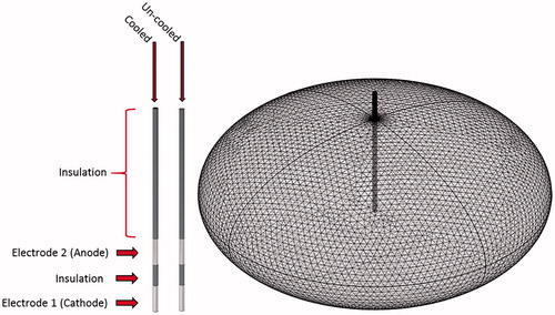
Table 1. Properties used within numerical model.

Material	Parameter	Value	Units	Reference
Liver	ρ, Density	1079	$\left[\mathrm{k}\mathrm{g}/{\mathrm{m}}^3\right]$	[10]
	$c_p,$ Heat capacity	3540	$\left[\mathrm{J}/\mathrm{k}\mathrm{g}/\mathrm{K}\right]$	[10]
	$k,$ Thermal conductivity	0.52	$\left[\mathrm{W}/\mathrm{m}/\mathrm{K}\right]$	[10]
	$\alpha$, Thermal coefficient of conductivity	2	$\left[\mathrm{\%}/°\mathrm{C}\right]$	[10]
	${\omega }_b$, Perfusion	${3.575e}^{-3}$	[1/s]	[10]
	$E_0,$ Reversible field threshold	460	$\left[\mathrm{V}/\mathrm{c}\mathrm{m}\right]$	[11]
	$E_1,$ Irreversible field threshold	700	$\left[\mathrm{V}/\mathrm{c}\mathrm{m}\right]$	[11]
Insulation	ρ, Density	2329	$\left[\mathrm{k}\mathrm{g}/{\mathrm{m}}^3\right]$	[10]
	$c_p,$ Heat capacity	700	$\left[\mathrm{J}/\mathrm{k}\mathrm{g}/\mathrm{K}\right]$	[10]
	$k,$ Thermal conductivity	130	$\left[\mathrm{W}/\mathrm{m}/\mathrm{K}\right]$	[10]
	$\sigma ,$ Electrical conductivity	${1.0e}^{-12}$	$\left[\mathrm{S}/\mathrm{m}\right]$	[10]
Electrode	ρ, Density	7900	$\left[\mathrm{k}\mathrm{g}/{\mathrm{m}}^3\right]$	[10]
	$c_p,$ Heat capacity	500	$\left[\mathrm{J}/\mathrm{k}\mathrm{g}/\mathrm{K}\right]$	[10]
	$k,$ Thermal conductivity	15	$\left[\mathrm{W}/\mathrm{m}/\mathrm{K}\right]$	[10]
	$\sigma ,$ Electrical conductivity	${2.22e}^{-6}$	$\left[\mathrm{S}/\mathrm{m}\right]$	[10]

Table 2. Comparison between the numerical model and actual experimental results for the initial and final current, as well as the root mean square error for the temperature trend throughout the 300 s treatment.

Metric	Initial current [A]	Final current [A]	RMSE for temperature [°C]
Un-cooled experimental	15.08 ± 2.66	29.20 ± 6.54	0.88
Un-cooled model	16.43	27.98
Cooled experimental	16 ± 2.07	26.37 ± 7.91	2.3
Cooled model	16.45	19.93

The initial conductivity and max-conductivity were set to 0.12 and 0.42 S/m, respectively to obtain the best possible fit. Figure 4 illustrates the transient temperature comparison for three different perfusion rates.

Figure 2. (A) An internally perfused bipolar applicator and the attached fiber optic temperature sensor. (B) A perfused porcine liver post treatment. Each treatment point was marked with stainless steel flags to serve as a guide during sectioning. (C) A representative schematic of the POM and pulse delivery system where, (1) perfused porcine liver, (2 and 3) hepatic artery and portal vein as inlets, (4) vena cava as outlet, (5) container, (6) filter, (7) heater/cooler system, (8) pump, (9) waveform generator, (10) IRE probe with fiber optic probe attached (shown as bipolar probe), (11) flask of deionized water, (12) peristaltic pump, (13) NanoKnife™ pulse generator, (14) fiber optic probe controller, (15) computer for temperature measurement acquisition. Overall, items 1–9 are integrated into the VasoWave™ organ preservation system, while items 10 and 13 are used for delivering IRE treatment, and 14, and 15 are for temperature measurement.

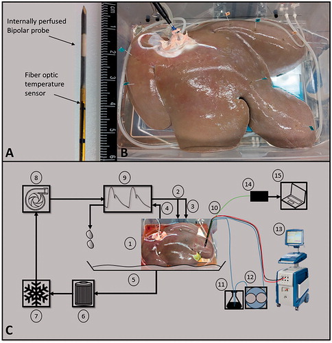
Table 3. Summary of the treatment parameters for the study of internal electrode cooling on electrical current, temperature, and treatment zone size.

								N
Parameter set	Electrode separation [cm]	Electrode exposure [cm]	Pulse amplitude [V]	No. pulses	Pulse length	Delivery rate [min^−1]	Generator	Cooled	Un-cooled
1	0.8	1	2700	300	100	90	BTX	5	5
2	0.8	1	2700–3000	400	100	90	NanoKnife	39	21

Figure 3. The (A, D) electrical field [V/cm], (B, E) temperature distribution [°C], and (C, F) thermal damage [%] for an IRE treatment in liver with solid un-cooled bipolar electrodes (top), and internally cooled bipolar electrodes at 26 °C (bottom). The results are shown in the z–x plane after 300 pulses were applied at 2700 V and a pulse with of 100 μs. The electrode exposure and spacing was 1 cm and 0.8 cm, respectively.

Figure 4. Illustrates the average measured thermal disparity (n = 5) for the cooled and un-cooled applicators over the course of treatment and compares to the numerically calculated temperature sequence for the same treatment protocol. Three different values of perfusion were modeled and the RMSE was taken to help quantify a closeness of fit between the measured and modeled results. (A) Shows perfusion at a physiologic level, ωb = 7.15e⁻³[1/s], and which illustrated an under-estimation of the measured temperature trend (${\mathrm{R}\mathrm{M}\mathrm{S}\mathrm{E}}_{\mathrm{c}\mathrm{o}\mathrm{o}\mathrm{l}\mathrm{e}\mathrm{d}}=2.15\hspace{0.17em}°\mathrm{C},{\mathrm{R}\mathrm{M}\mathrm{S}\mathrm{E}}_{\mathrm{u}\mathrm{n}\mathrm{c}\mathrm{o}\mathrm{o}\mathrm{l}\mathrm{e}\mathrm{d}}=1.6\hspace{0.17em}°\mathrm{C})$. (B) Perfusion at 50% of the physiologic level, ωb = 3.575e⁻³ [1/s], and results in a close approximation$\hspace{0.17em}({\mathrm{R}\mathrm{M}\mathrm{S}\mathrm{E}}_{\mathrm{c}\mathrm{o}\mathrm{o}\mathrm{l}\mathrm{e}\mathrm{d}}=2.3\hspace{0.17em}°\mathrm{C},{\mathrm{R}\mathrm{M}\mathrm{S}\mathrm{E}}_{\mathrm{u}\mathrm{n}\mathrm{c}\mathrm{o}\mathrm{o}\mathrm{l}\mathrm{e}\mathrm{d}}=0.88\hspace{0.17em}°\mathrm{C})$. (C) Shows perfusion at 20% of the physiologic level, ωb = 1.43e⁻³ [1/s], and provided an over-estimation of the temperature trend$\hspace{0.17em}({\mathrm{R}\mathrm{M}\mathrm{S}\mathrm{E}}_{\mathrm{c}\mathrm{o}\mathrm{o}\mathrm{l}\mathrm{e}\mathrm{d}}=2.5\hspace{0.17em}°\mathrm{C},\hspace{0.17em}{\mathrm{R}\mathrm{M}\mathrm{S}\mathrm{E}}_{\mathrm{u}\mathrm{n}\mathrm{c}\mathrm{o}\mathrm{o}\mathrm{l}\mathrm{e}\mathrm{d}}=1.74\hspace{0.17em}°\mathrm{C})$. Interestingly, varying the perfusion within the numerical model had little effect on the cooled applicator scenario.

Figure 5. A comparison of gross pathology of treatment zones using (A) an internally cooled bipolar applicator and (B) an un-cooled applicator during the same IRE treatment protocol. Figure 3(B) clearly presents a centrally located white coagulated region as a result of thermal damage to the tissue, while Figure 3(A) shows much less thermally damaged tissue. Both images were taken prior the use of any staining.

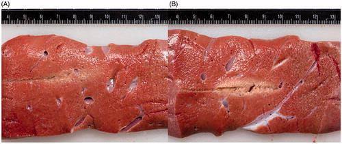
Figure 6. The effect of internal electrode cooling for fixed-amplitude IRE treatments. (A) A comparison of the initial and final electrical current measurements for cooled and un-cooled applicator designs shows an overall increase in current throughout treatment. Focusing on the final current measurement taken after the last pulse of treatment, the internally cooled applicator generated 26.32 ± 6.54 A, while the un-cooled generated 29.20 ± 7.91 A on average. (B) Initial and final temperature measurements were also compared to show the overall increase in tissue temperature throughout the treatments. The final temperature measurement differed by between the cooled and un-cooled applicator by 9.42 ± 1.4 °C (cooled 33.01 ± 1.7 °C, un-cooled 42.43 ± 3.1 °C) ($p\le .0001$). (C) Both the long and short axes were measured and compared for the cooled and un-cooled applicators, generating an average treatment zone size of 3.88 ± 0.25 cm by 2.08 ± 0.33 cm for the cooled applicator and a 3.86 ± 0.44 cm by 2.12 ± 0.63 cm treatment zone for the uncooled applicator.

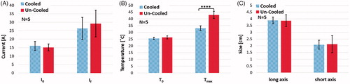
Figure 7. This plot illustrates the measured voltage and current for a specific un-cooled treatment. The arrow denotes where the voltage was stepped down from 3000 to 2900 V, approximately 150 s into the treatment.

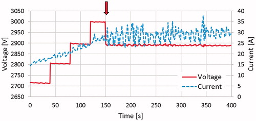
Figure 8. Comparison of average (a) voltage amplitude, (b) electric current, and (c) delivered electric power during the treatments with cooled and un-cooled bipolar applicators. Upon reaching the target amplitude of 3000 V, the un-cooled applicators showed an immediate declination in voltage amplitude, descending to 2900 V only 100 pulses later and finishing at 2834 V due to electrical arching. The internally cooled electrical applicators maintained the target amplitude of 3000 V for a while longer before experiencing more significant arching, and eventually finishing at 2880 V. In response to the arc-mitigation software, the average electrical current and power generated are maintained at a suitable level, though the internally cooled applicators consistently showed less current and power, while still delivering pulsed electric fields at a higher voltage.

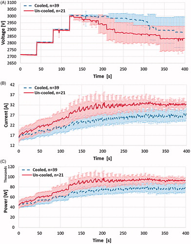
Figure 9. The effect of internal electrode cooling for ramped-amplitude IRE treatments using the NanoKnife™ arc-mitigation system. (a) A comparison of the initial and final electrical current measurements for cooled and un-cooled applicator designs, shows an overall increase in current throughout treatment. Focusing on the final current measurement taken after the last pulse of treatment, the internally cooled applicator generated 41.07 ± 7.48 A, while the un-cooled applicator generated 47.20 ± 3.12 A on average ($p\le .001$). (b) Initial and final temperature measurements were also compared to show the overall increase in tissue temperature throughout the treatments. The final temperature measurement differed between the cooled and un-cooled applicator by 9.97 ± 3.98 °C (cooled 34.93 ± 4.06 °C, un-cooled 44.9 ± 8.04 °C) ($p\le .005$). (c) The average treatment zone dimensions were 3.67 ± 0.71 cm by 2.27 ± 0.48 cm for the cooled applicator and 3.58 ± 0.72 cm by 2.09 ± 0.57 cm for the uncooled applicator.

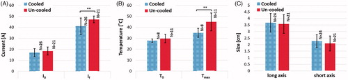
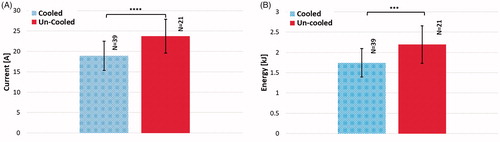
Figure 10. Comparison of (A) average current and (B) average delivered energy during treatments with cooled and un-cooled applicators ($p\le .005$, $p\le .005$).

Hasgall P, Di Gennaro F, Baumgartner C, et al. IT’IS Database for thermal and electromagnetic parameters of biological tissues, Version 3.0. 2015. [Online]. Available from: www.itis.ethz.ch/database

 Google Scholar

SelCukjati D, Batiuskaite D, Slivnik DT, et al. Sequential finite element model of tissue electropermeabilisation. 26th Annu Int Conf IEEE Eng Med Biol Soc. 2004;4:3551–3554.

 Google Scholar