Figures & data
Figure 1. (a) Internally cooled-wet (ICW) electrode used in the clinical trial. (b) Electrode scheme and dimensions (in mm, out of scale). Blue arrows indicate the internal flow of cooling liquid while red arrows show the outflow of hypertonic saline through expandable needles. (c) Geometry of the three-compartment model used in the computational study. Note that the geometry of infused tissue is for illustrative purposes only, i.e. it does not coincide with the contour geometry of saline-infused tissue computed from the “generic pattern” (shown in Figure 2(b,c), respectively).
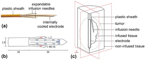
Table 1. Characteristics of the materials used in the computational model (references in brackets).
Figure 2. (a) Images of saline spatial distribution from the six saline injection trials (1 – 6) conducted on the in vivo model. Saline presence is shown in white, while electrode, infusion needles and noninfused tissue are in black. (b) “Generic pattern” of saline spatial distribution derived from the six images from (a) by thresholding and merging them into one greyscale image. (c) Contour geometry of saline-infused tissue derived from the “generic pattern” in (d) and used in the computer model.
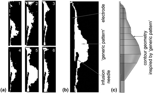
Figure 3. Impedance evolution in the six analysed cases: A (one-compartment model, only liver), B (two-compartment model, with liver and saline-infused liver using the saline distribution with spherical geometry as proposed in [Citation13]), C (two-compartment model, with healthy liver and saline-infused healthy liver using the saline spatial distribution obtained from the in vivo experiment), D (two-compartment model, with non-infused healthy liver and tumour), E (three-compartment model, with healthy liver, tumour with noninfused and saline-infused zones, and spherical geometry infusion) and F (three-compartment model, with healthy liver, tumour with noninfused and saline-infused zones, and saline spatial distribution obtained from the in vivo experiment). The horizontal grey band represents the range of impedance values observed in the clinical trial. Roll-off time is shown for cases A, B and D.
![Figure 3. Impedance evolution in the six analysed cases: A (one-compartment model, only liver), B (two-compartment model, with liver and saline-infused liver using the saline distribution with spherical geometry as proposed in [Citation13]), C (two-compartment model, with healthy liver and saline-infused healthy liver using the saline spatial distribution obtained from the in vivo experiment), D (two-compartment model, with non-infused healthy liver and tumour), E (three-compartment model, with healthy liver, tumour with noninfused and saline-infused zones, and spherical geometry infusion) and F (three-compartment model, with healthy liver, tumour with noninfused and saline-infused zones, and saline spatial distribution obtained from the in vivo experiment). The horizontal grey band represents the range of impedance values observed in the clinical trial. Roll-off time is shown for cases A, B and D.](/cms/asset/0087834a-0e22-4970-8154-f6987d8d33e8/ihyt_a_1489071_f0003_b.jpg)
Figure 4. Joule heat distribution in the tissue for cases A–F at 1 s of ablation, (logarithmic scale in W/m3). Note that maximum values are reached only on the electrode surface and the infusion needles.
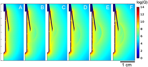
Figure 5. a: Temperature profiles of cases A–E. Black and white contours are 50 °C and 100 °C isotherms, respectively. The transversal diameter value and time of acquisition are shown in all cases at roll-off times before 240 s or at 240 s in the absence of roll-off. b: Detail of electrode zone in (a) with 100 °C white isotherm shown.
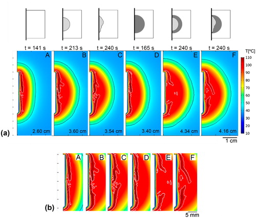
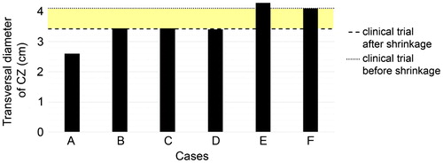
Figure 6. Transversal diameters of the coagulation zones computed for the considered cases A–F. Horizontal lines are the mean transversal diameter found in the clinical trials (dashed line) and the “corrected value” by taking the shrinkage effect into account (dotted line). The coloured band thus represents the range in which the clinical and computed results would match.