Estimation of the temperature field in laser-induced hyperthermia experiments with a phantom

Figures & data

Figure 1. X-ray powder diffraction patterns.

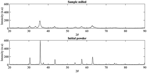
Figure 2. FEG-SEM micrographs of the milled sample.

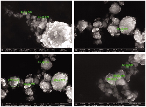
Figure 3. (a) Top view of the phantom with thermocouples; (b) Experimental setup; (c) Snapshot of the infra-red camera readings.

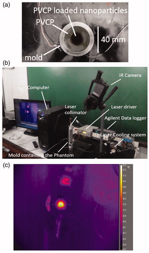
Figure 4. Sketch of the phantom with its associated dimensions, laser beam, thermocouples and IR camera.

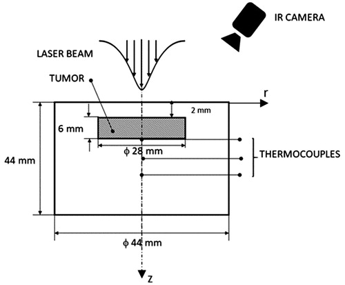
Table 1. Liu and West’s algorithm [28].

Step 1

Find the mean ${\overline{\mathbf{\theta }}}_{k-1}$ of the parameters $\mathbf{\theta }$ at time tk–1.

Step 2

For i = 1,…,N compute ${\mathbf{m}}_{k-1}^i$ with Equation (7)(7) $${\mathbf{m}}_{k-1}^i=A\hspace{0.17em}\hspace{0.17em} {\mathbf{\theta }}_{k-1}^i+(1-A) {\overline{\mathbf{\theta }}}_{k-1}$$(7) , draw new particles ${\mathbf{x}}_k^i$ from the prior density π(xk|${\mathbf{x}}_{{{}_k}_{-1}}^i$,${\mathrm{m}}_{k-1}^i$) and then calculate the mean ${\mu }_k^i$ of xk. Use the likelihood density to calculate the corresponding weights w^ik = π(zk|${\mathbf{\mu }}_k^i$,${\mathbf{m}}_{k-1}^i$)w^ik–1.

Step 3

Calculate the total weight t = Σi w^ik and then normalise the particle weights, that is, for i = 1,…, N let w^ik = t^–1 w^ik .

Step 4

Resample the particles as follows:

Construct the cumulative sum of weights (CSW) by computing ci = ci–1 + w^ik for i = 1,…, N, with c0 = 0

Let i = 1 and draw a starting point u1 from the uniform distribution U[0,N^-1]

For j = 1,…,N

Move along the CSW by making uj = u1 + N^−1(j−1)

While uj > ci make i = i + 1

Assign samples ${\mathbf{x}}_{{{}_k}_{-1}}^j={\mathbf{x}}_{{{}_k}_{-1}}^i$, ${\mathbf{m}}_{{{}_k}_{-1}}^j={\mathbf{m}}_{{{}_k}_{-1}}^i$and ${\mathbf{\mu }}_{{}_k}^j={\mathbf{\mu }}_{{}_k}^i$

Assign parent ij = i

Step 5

For j = 1,…, N draw samples ${\mathbf{\theta }}_k^j$ from $N({\mathbf{\theta }}_k^j|{\mathbf{m}}_{k-1}^{ij},h^2{\mathbf{V}}_{k-1})$, by using the parent ij

Step 6

For j = 1,…, N draw particles ${\mathbf{x}}_{{}_k}^j$ from the prior density π(xk|${\mathbf{x}}_{{}_{k-1}}^{ij}$,${\mathbf{\theta }}_k^j$), by using the parent ij, and then use the likelihood density to calculate the correspondent weights $w_k^j$ = π(zk|${\mathbf{x}}_k^j$,${\mathbf{\theta }}_k^j$)/π(zk|${\mathbf{\mu }}_{{}_k}^{ij}$,${\mathbf{m}}_{{}_{k-1}}^{ij}$)

Step 7

Calculate the total weight t = Σj$w_k^j$ and then normalise the particle weights, that is, for j = 1,…, N let $w_k^j$ = t^–1 $w_k^j$

Table 2. Means for the priors of the model parameters.

Parameter	PVCP	PVCP with nanoparticles
k0 (Wm^–1K^–1)^a	0.21	0.22
C0 (Jm^–3K^–1)^b	1.4989 × 10^6	1.4755 × 10^6
κ0 (m^–1)	9^c	125^d
h0 (Wm^–2K^–1)^e	10
E01 (Wm^–2)^f	4580.5
E02 (Wm^–2)^f	6447.7

^a Measured in this work with C-Therm TCi thermal conductivity analyzer.

^bDirectly calculated with thermal conductivity and thermal effusivity measured in this work.

^c References [41,42].

^d Estimated in this work from independent surface temperature measurements in the heated phantom.

^e Natural convection with air and linearized radiation at room temperature.

^f Directly calculated with laser power and beam radius measured in this work.

Figure 5. Comparison of the measured and estimated transient temperature variations at (r = 0, z = 8) mm: (a) Laser power P₁; (b) Laser power P₂.

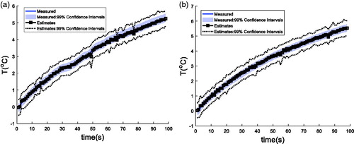
Figure 6. Comparison of the measured and estimated transient temperature variations at (r = 0, z = 10) mm: (a) Laser power P₁; (b) Laser power P₂.

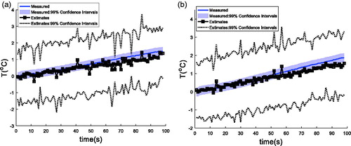
Figure 7. Comparison of the estimated radial temperature variation with the measurements obtained at z = 0 with an infra-red camera at selected times (t = 60 s: top; t = 90s: bottom). Experiment with P₁ (left) and P₂ (right).

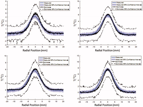
Figure 8. Estimated temperature variation on a longitudinal cut through the centre of the phantom at t = 90 s: (a) Laser power P₁; (b) Laser power P₂.

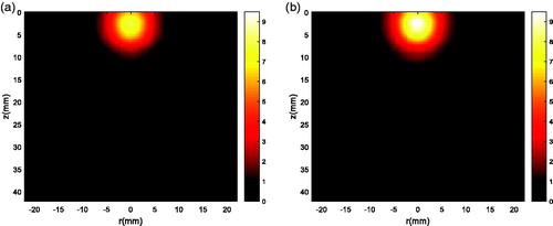
Figure 9. Estimated fluence rates on a longitudinal cut through the centre of the phantom at t = 90 s: (a) Laser power P₁; (b) Laser power P₂.

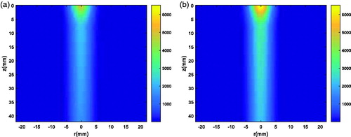
Figure 10. Confidence intervals (99%) of the model parameters sequentially estimated with the particle filter: Experiments with P₁ (red) and P₂ (blue). Initial prior mean is shown by the grey line.

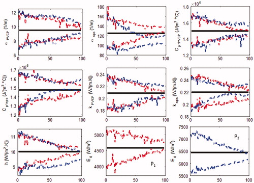
Table 3. Model parameters estimated at the final time t = 100 s.

			P1 = 156.6 mW		P2 = 220 mW
Parameter	Material	Prior Mean	Estimated Mean	Estimated 99% Confidence Interval	Estimated Mean	Estimated 99% Confidence Interval
k (W m^−1 K^–1)	PVCP	0.21	0.206	(0.201,0.211)	0.213	(0.206,0.219)
	PVCP with Fe2O3 NP	0.22	0.216	(0.209,0.222)	0.225	(0.216,0.234)
C (J m^−3 K^–1) × 10^–6	PVCP	1.4989	1.48	(1.46,1.50)	1.51	(1.46,1.56)
	PVCP with Fe2O3 NP	1.4755	1.50	(1.46,1.53)	1.54	(1.48,1.59)
κ (m^–1)	PVCP	9	9.2	(8.5,9.9)	9.7	(9.1,10.4)
	PVCP with Fe2O3 NP	125	133	(128,137)	113	(105,121)
h (W m^−2 K^–1)	—	10	10.1	(9.9,10.3)	9.8	(9.5,10.0)
E1 (Wm^–2)	—	4580.5	4645	(4519,4771)	—	—
E2 (Wm^–2)	—	6447.7	—	—	6282	(6162,6404)

Liu J, West M. Combined parameter and state estimation in simulation-based filtering. In: De Freitas JFG, Doucet, A, Gordon NJ, editors. Sequential Monte Carlo Methods in Practice. New York (NY): Springer-Verlag; 2001. pp. 197–223.

 Google Scholar

Fonseca M, Zeqiri B, Beard P, et al. Characterisation of a PVCP-based tissue-mimicking phantom for quantitative photoacoustic imaging. Proc SPIE Opto-Acoustic Methods Appl Biophotonics II. 2015;9539:953911.

 Google Scholar

Jeong EJ, Song HW, Lee YJ, et al. Fabrication and characterization of PVCP human breast tissue-mimicking phantom for photoacoustic imaging. Biochip J. 2017;11:67–75.

 Web of Science ®Google Scholar