Numerical analysis of thermal response of tissues subjected to high intensity focused ultrasound

Figures & data

Figure 1. (a) Schematic of the HIFU-subjected tissue phantom geometry for simulations. (b) Schematics of ZX plane (axis-symmetric along z-axis) around y = 0: (b.i) two-layered medium, (b.ii) multi-layered medium and (b.iii) multi-layered with inhomogeneity. (c) Boundary conditions for pressure (c.i) and temperature (c.ii). (All dimensions are in cm).

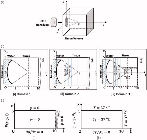
Table 1. Transducer Parameters.

Symbol	Property	Value
$a$	Radius of transducer (Aperture = $2a$)	3.5 cm
$d$	Focal length (Transducer radius of curvature)	7.0 cm
$f_0$	Transducer frequency	1.0 MHz

Table 2. Acoustic and thermo-physical properties.

Symbol	Properties	Unit	Water	Skin	Fat	Muscle	Liver tissue	Blood
$c_0$	Speed of sound	m/s	1520	1540	1430	1560	1570	1540
${\rho }_0$	Density of material	kg/m^3	1000	1100	910	1050	1055	1060
${\alpha }_0$	Attenuation coefficient	Np/m	0.026	16	7	9	8.1	1.5
$\beta$	Nonlinearity coeff.		3.5	4.9	6.5	4.5	4.5	4.0
k	Thermal conductivity	W/m °C	0.6	0.28	0.24	0.51	0.51	0.53
Cp	Heat capacity	J/kg °C	4200	3500	3800	3700	3600	3770
ωb	Volumetric Blood perfusion rate	kg/m^3s	0	0	0	0.5	10	–

Figure 2. Pressure variation with respect to axial direction (along the direction of propagation of the ultrasound waves) for different grid sizes in space (a) for different dz (b) for different dx, to optimise the discretized step size in space.

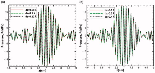
Figure 3. Comparison of the numerical solution of Westervelt equation as obtained in the present work with that of the analytical Rayleigh integral solution given by Hamilton [28]; (a) time and (b) space variation of acoustic pressure in water medium.

Figure 4. Nonlinear peak positive and peak negative pressure distribution compared with linear pressure distribution (a) with respect to time and (b) along the axial distance, (c) volumetric heat generation and (d) temperature distribution along the axial distance.

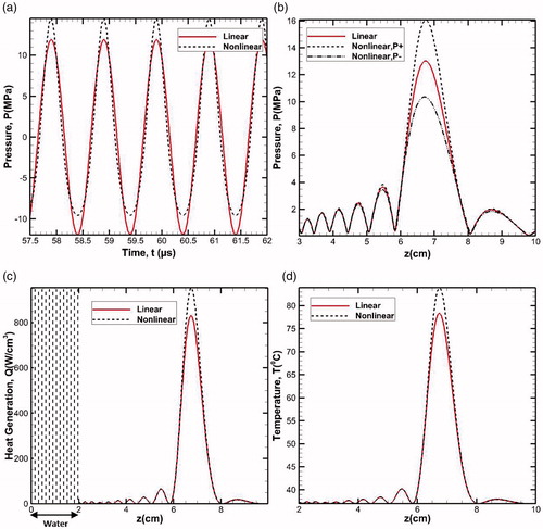
Figure 5. Intensity plot along the axial distance for different domains. The layer consists of skin (0.2 cm) + fat (1 cm) + muscle (1.5 cm). In all the cases, 2 cm of water is placed between transducer and the medium.

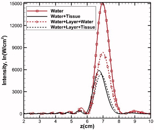
Table 3. Quantitative analysis of various medium intensity.

Medium	zfocalplane (cm)	In (W/cm^2)
Water	6.9616	15148.7
W + Tissue	6.7488	5886.36
W + L+Water	6.992	8383.46
W + L+Tissue	6.8552	5387.41

Figure 6. Intensity plots along the axial distance to show the effect of single layer (fat/muscle) sandwiched between (a) two layers of water and (b) water and liver tissue. For better clarity, the layer configurations have schematically been shown in both the figures.

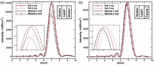
Figure 7. Temperature contour plots in the focal plane (z-x plane) for varying fundamental frequencies (0.8, 1 and 1.2 MHz) and of varying source pressures (0.2, 0.5 and 0.7 MPa).

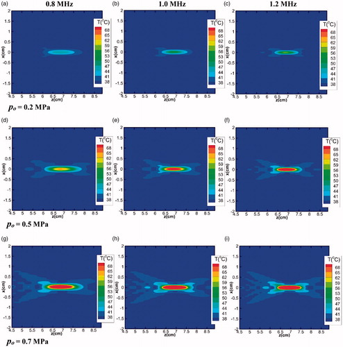
Figure 8. Temperature contour plots in the x-y plane for the focus point (z = 7 cm) for different fundamental frequencies (a) 0.8 MHz, (b) 1 MHz and (c) 1.2 MHz. For each case, the source pressure has been taken 0.5 MPa and heating duration is 0.2 s.

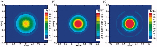
Figure 9. Temperature variation along the axial direction for different frequencies.

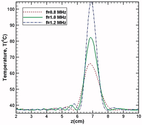
Figure 10. Generation of multiple lesions: (a) 1 lesion (b) 2 lesions (c) 3 lesions and (d) 5 lesions. First, second and the third column respectively represent the volumetric power, corresponding transient temperature and thermal dosage for each lesion. In the contours shown, L_i (i = 1, 2, ., 5) represents the number of the lesion created.

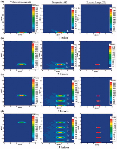
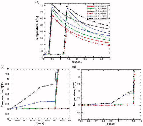
Figure 11. Temperature for m = 1, $m\times \mathit{\text{heating}}\mathit{\text{ time}}$ and $m\times \mathit{\text{volumetric}}\mathit{\text{ power}}$ for different lesions (a) with respect to time, (b) along the axial direction.

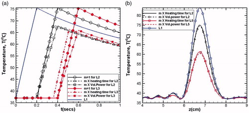
Figure 12. Delay time period in (a) modulation of volumetric power generation, and (b) modulation of heating time.

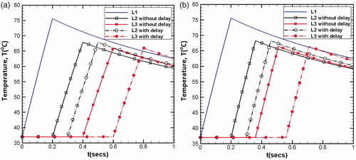
Figure 13. Effect of total number of lesions on the resultant temperature distributions realised in the x-z (left column) and x-y planes (right column).

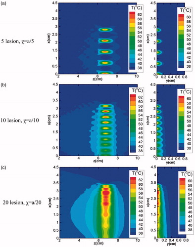
Figure 14. Temperature at the focus point for (a) lesion 2 and lesion 5 for total number of lesions 5, 10 and 20, enlarged version (b) for lesion 2 (L₂) (c) for lesion 5 (L₅) shows the preheating time.

Hamilton MF. Comparison of three transient solutions for the axial pressure in a focused sound beam. J Acoust Soc Am. 1992;92:527–532.

 Web of Science ®Google Scholar