A new microwave applicator for laparoscopic and robotic liver resection

Figures & data

Figure 1. (a) Schematic of the proposed device. (b) Internal mechanical structure. (c) Computational domain configuration in CST: (1) internal temperature of the needle; (2), (3) reference points for validation through thermo-camera measurements. (d) Computational domain configuration in solidworks flow simulation (SFS): (1) internal temperature of input needle obtained through CST results; (4) output reference point for validation through thermocouple measurements.

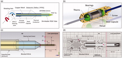
Figure 2. (a) Schematic description of the proposed procedure and its (b) laboratory setup, (c) real prototype in a bent state.

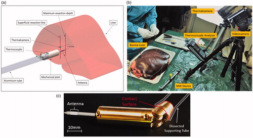
Table 1. Physical properties of hepatic tissue at 2.45 GHz frequency+.

Property	Value
Name	Liver
Density	1020 kg/m^3
Specific heat	3600 J/(kg*K)
Dielectric constant	53
Electrical conductivity	1.73 S/m
Thermal conductivity	0.469 W/(m*K)

Table 2. Protocol duty cycle.

Protocol	On [s]	Off [s]
1°	20	30
2°	30	30
3°	40	30

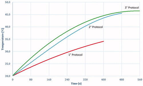
Figure 3. Temperature evolution results obtained through the CST simulator.

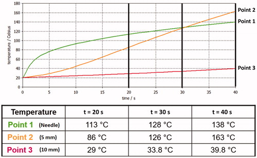
Figure 4. Isothermal distributions on the Y–Z plane of protocols coupled thermal EM simulations.

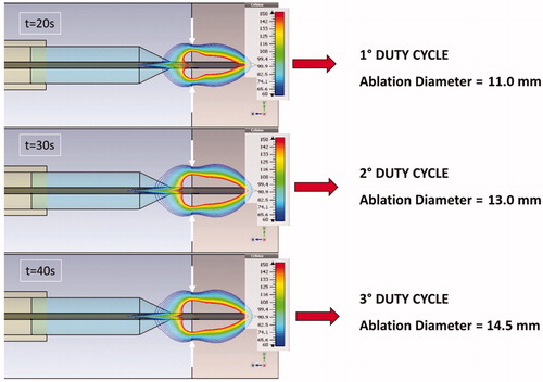
Figure 5. Temperature evolution at Point 1(Figure 1(d)) for different protocols (HPh: red boxes, CPh: blue boxes).

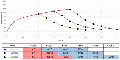
Figure 6. Temperature evolution at Point 4 (Figure 1(d)) for different protocols (HPh: red boxes, CPh: blue boxes).

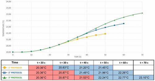
Figure 7. Isothermal distributions on the Y–Z plane of the thermal field on SFS.

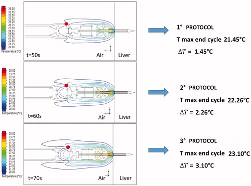
Figure 8. Protocols ablation series: (a) difference in the superficial radius dimensions in each protocol; (b) Thermal image at the end of eight sequential ablations using the 1°-protocol.

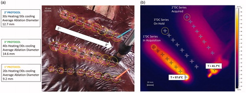
Figure 9. Coagulated area after eight ablations: dimensional references refer to the 2° protocol.

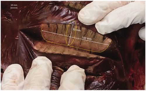
Figure 10. Mean statistical temperature evolution measured using the thermal camera: orange and red curves represent temperature evolution at points 2 and 3, respectively.

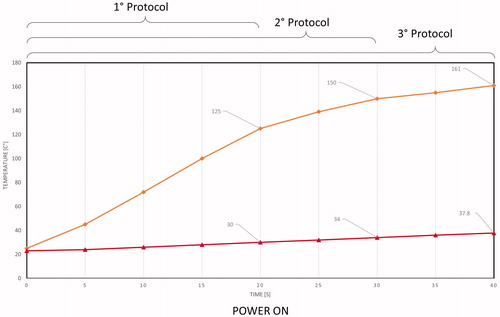
Figure 11. Average temperature evolution measured using the thermocouple: the yellow, blue, and green lines represent the temperature evolution for 1°, 2°, and 3° protocols.

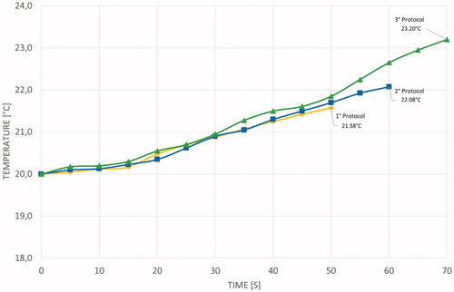
Figure 12. Comparison of results of simulated protocols at points 2 and 3 for the Power-ON phase.

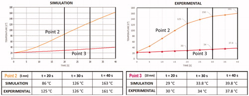
Figure 13. Comparison between results of simulated protocols (green) and experimental protocols (red) at Point 4.

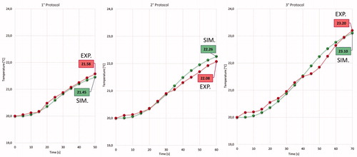
Figure 14. Temperature evolution during the eight sequential ablation measured on point 4 (Figure 1(d)): 1° protocol (Red); 2° protocol (Blue); 3° protocol (Green).