Comparison of temperature change and resulting ablation size induced by a 902–928 MHz and a 2450 MHz microwave ablation system in in-vivo porcine kidneys

Figures & data

Figure 1. MWA in in-vivo porcine kidneys with fiber optic thermal sensors inserted through the acrylic apparatus perpendicular to the microwave antenna axis plane.

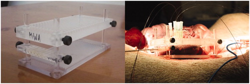
Figure 2. Location of the fiber optic thermal sensors relative to the MWA antenna axis (center of grid) for the (a) 902–928 MHz system and the (b) 2450 MHz system.

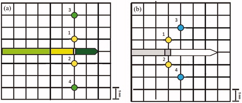
Figure 3. Example of the temperature change as a function of time during MWA in in-vivo porcine kidneys. The initial temperature rise can be described by a power equation. Following the inflection point, an exponential equation best fits the temperature changes. (Adapted from temperatures measured at 5 mm from the MWA antenna during an ablation using the Acculis 2450 MHz system).

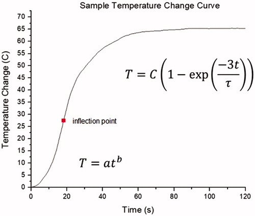
Figure 4. Sample non-linear regression of temperature increases using the power equation (Equation (1)(1) $$\Delta T\left(t\right)=a{t}^b,$$(1) ) for the initial 10 s of MWA using the (a) 902–928 MHz system and the (b) 2450 MHz system at 5 mm from the microwave antenna axis.

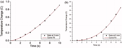
Figure 5. Non-linear regression of temperature increases at 5 mm during MWA using the (a) 902–928 MHz system and the (b) 2450 MHz system performed after the inflection point (Equation (2)(2) $$\Delta T\left(t\right)=C\left(1-\exp \left(\frac{-3t}{\tau }\right)\right),$$(2) ).

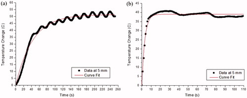
Table 1. Non-linear regression parameters for temperature changes during the initial 10 s of ablation at 5 mm from the antenna axis.

System	Maximum temperature after 10 s (°C)	a	b	R-squared
902–928 MHz	37.09 ± 1.06	0.0299 ± 0.027	1.910 ± 0.372	0.999 ± 0.001
2450 MHz	51.64 ± 15.31	0.1598 ± 0.158	2.039 ± 0.366	0.999 ± 0.001

Table 2. Non-linear regression parameters for temperature changes following the time of inflection at 5 mm from the antenna axis.

System	Temperature at inflection (°C)	Time of inflection (s)	C	τ	R-squared
902–928 MHz	39.13 ± 2.83	42.79 ± 8.80	46.36 ± 9.90	184.73 ± 92.98	0.93 ± 0.07
2450 MHz	62.73 ± 8.50	23.99 ± 26.64	45.48 ± 8.57	47.80 ± 60.39	0.98 ± 0.01

Table 3. Time to achieve 99.99% cell damage at each thermal sensor location during MWA using a 902–928 MHz and a 2450 MHz system.

	Time to 99.99% (s)
System	Thermal sensor 1	Thermal sensor 2	Thermal sensor 3	Thermal sensor 4
902–928 MHz	75.01 ± 16.69	172.19 ± 89.73	607.48 ± 102.40	99.99% not achieved
2450 MHz	23.84 ± 12.49	38.15 ± 29.73	81.32 ± 36.26	84.66 ± 25.73

Table 4. Ablation size and circularity following MWA using a 902–928 MHz and a 2450 MHz system.

System	Long axis diameter (cm)	Short axis diameter (cm)	Circularity
902–928 MHz	3.33 ± 0.67	2.40 ± 0.54	0.72 ± 0.06
2450 MHz	4.09 ± 0.89	3.32 ± 0.41	0.83 ± 0.12