Real-time monitoring radiofrequency ablation using tree-based ensemble learning models

Figures & data

Figure 1. (a) The RFA tissue setup is shown with temperature probes inserted into each face of the device. (b) The RFA device is shown, with electrodes grouped by face. (c) The RFA device face partitioning on the surface of the device. (d) The new instrumentation system is shown, with the red box showing the RF generator connection socket, the green box showing the relay-based electrode switching subsystem, the yellow box showing the impedance analyzer subsystem, the orange box showing an auxiliary temperature measurement subsystem, and the purple box showing the RFA device connection socket.

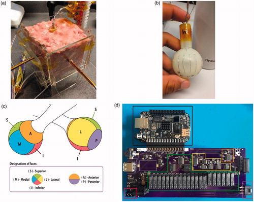
Table 1. Number of data points and their distribution to different sets for regression data from both instrumentations.

	Number of data points
Dataset	Total	Training (at each fold)	Validation (at each fold)	Test
First Instrumentation	12480	7862	874	3744
Second Instrumentation	10344	6517	724	3103

Figure 2. The grid search for the hyperparameters of both ensemble models with a comparison between the datasets. The criterion for the best hyperparameter value is the test R². a) Tuning the maximum number of leaf nodes for Random Forest. (Number of trees fixed at 80 for both models). b) Tuning the number of trees for Random Forest. (Max. number of leaf nodes fixed at 250 and 900 for the first and second instrumentation, respectively). c) Tuning the maximum number of leaf nodes for Adaptive Boosting. (Number of trees fixed at 30 for both models). d) Tuning the number of trees for Adaptive Boosting. (Max. number of leaf nodes fixed at 250 and 700 for the first and second instrumentation, respectively).

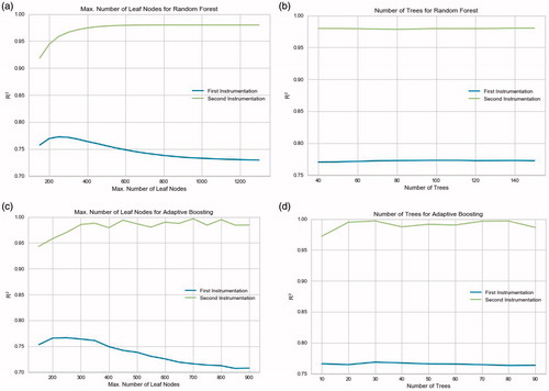
Table 2. Output performances of all the ML models when cross-validated and tested on the first instrumentation data.

	Prediction metrics for regression
ML Model	Test RMSE (mm)	Test R^2	CV-average RMSE (mm)	CV-average R^2
ANN^a	2.45	68.1%	2.45	67.6%
Random Forest	2.16	77.2%	2.20	76.3%
Adaptive Boosting	2.08	79.3%	2.12	75.2%

Note: ^aThe same model and hyperparameters from [31].

Table 3. Output performances of all the ML models when cross-validated and tested on the second instrumentation data.

	Prediction metrics for regression
ML Model	Test RMSE (mm)	Test R^2	CV-average RMSE (mm)	CV-average R^2
ANN^a	2.19	57.0%	2.23	56.0%
Random Forest	0.54	98.0%	0.62	96.2%
Adaptive Boosting	0.30	99.1%	0.51	97.5%

Note: ^aThe same model and hyperparameters from [31].

Figure 3. Residual plots of the predictions of the ensemble models on the test data from both instrumentations. The 0.0 mm depth is the tissue directly abutting the surface of the RFA device face. a) Random Forest on the first instrumentation data. b) Random Forest on the second instrumentation data. c) Adaptive Boosting on the first instrumentation data. d) Adaptive Boosting on the second instrumentation data.

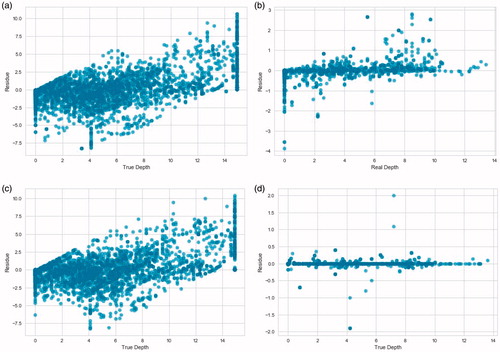
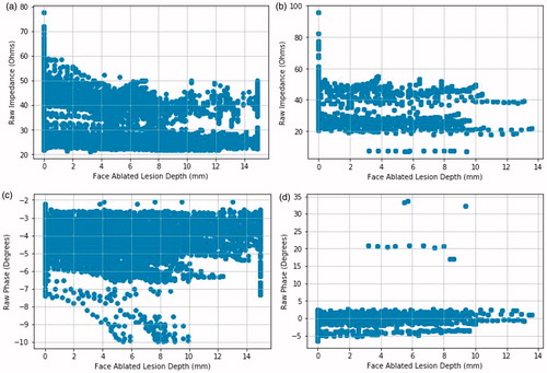
Figure 4. Magnitude and phase plots of datasets from both instrumentation setups. Face ablated lesion depth is the depth of the ablation lesion relative to a face of the RFA device. The 0.0 mm depth is the tissue directly abutting the surface of the RFA device face. a) Magnitude vs. depth for the first instrumentation. b) Magnitude vs. depth for the second instrumentation. c) Phase vs. depth for the first instrumentation. d) Phase vs. depth for the second instrumentation.

Wang YC, Chan TC, Sahakian AV. Real-time estimation of lesion depth and control of radiofrequency ablation within ex vivo animal tissues using a neural network. Int J Hyperther. 2018;34(7):1104–1113.

 Web of Science ®Google Scholar