Investigation of laser pulsing parameters’ importance in Er:YAG laser skin ablation: a theoretical study conducted via newly developed thermo-mechanical ablation model

Figures & data

Figure 1. Sketch illustrating the assumed skin’s tissue microstructure. Skin’s tissue water is assumed to be entrapped within a cylindrical cavity that is attached to a spring-piston compound. The cavity’s wall represents the tissue’s elastic solid medium.

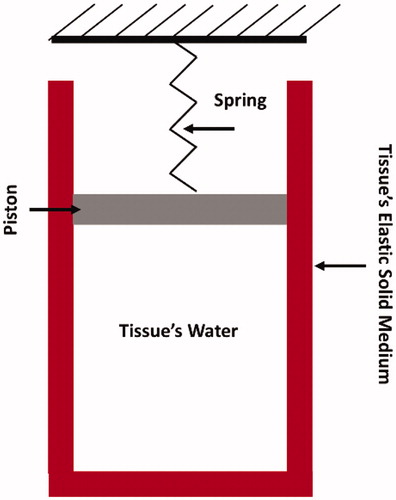
Table 1. Thermo-physical properties of skin tissue [37].

Property	Value
Water content (w)	65%
Density (ρtissue )	1100 kg m^−3
Thermal conductivity (k)	0.4 W m^−1 K^−1
Specific heat capacity of tissue’s solid medium (cs)	1670 J kg^−1 K^−1

Figure 2. The evolution of tissue’s relative volume (ratio of volume to initial volume), pressure, and temperature as a function of volumetric energy density in the tissue. The results are obtained using 10 J cm⁻² pulse fluence, 20 µs pulse duration, and 3000 cm⁻¹ absorption coefficient.

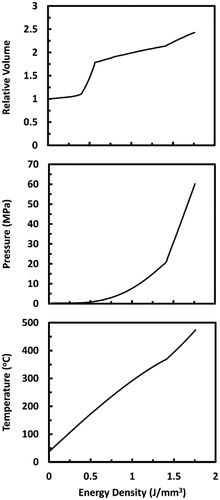
Figure 3. A sketch showing the discretization of the computational domain into N equal control volumes of size Δx. The dependent variables were solved at the spatial nodes placed in the center of the control volumes. Temperature profile between adjacent nodes was assumed to be linear.

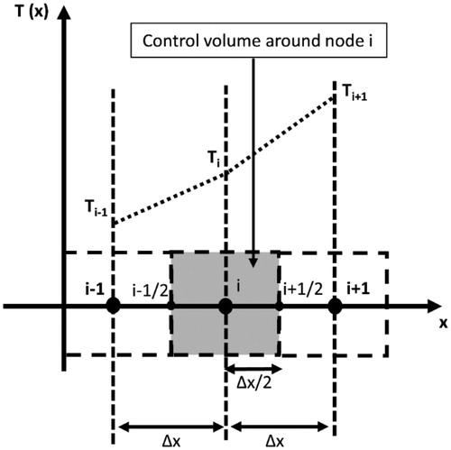
Figure 4. Verification of the computational model by comparing with the analytical model developed by Venugopalan et al. [26]. The comparison is made in terms of (a) temperature profile outside the vapor-liquid layer, (b) thickness of the vapor–liquid layer, and (c) tissue’s ablation front position as a function of time. Continuous wave Er:YAG laser with irradiance (I = 150 W cm⁻²) was applied. Spatial and temporal grid size of 1 µm and 5 µs, respectively, were utilized.

Figure 5. Validation of the computational model by comparing with experimental results extracted from Ref. [48]. The comparison is made in terms of tissue’s mass loss (ablation) as a function of pulse fluence. A pulse duration of 2 µs, a pulse frequency of 1 Hz, and an absorption coefficient of 400 cm⁻¹ are employed here.

Figure 6. Tissue temperatures as functions of time during and after a 200 µs long Er:YAG laser pulse at several selected depths within the tissue. The time is taken from the onset of irradiation. Pulse fluence is equal to 1.21 J cm⁻². Surface tissue temperature calculated while neglecting water phase change is added for comparison.

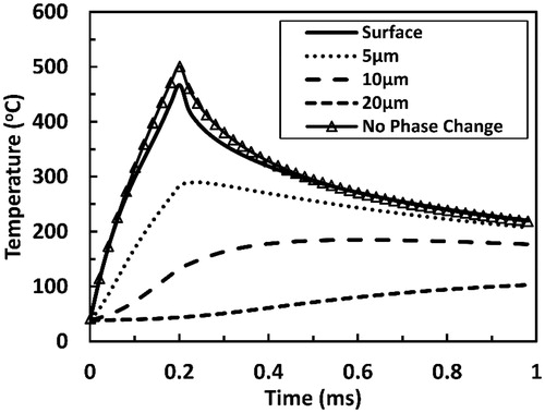
Figure 7. Temperature profiles predicted at several selected time points from the onset of laser tissue irradiation with a 200 µs long Er:YAG laser pulse. x represents the depth within the irradiated tissue with x = 0 indicating the surface. The pulse fluence is equal to 1.21 J cm⁻².

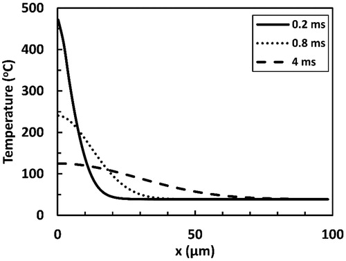
Figure 8. Predicted coagulation thickness as a function of time as a result of irradiation with a 200 µs long Er:YAG laser pulse. Two sub-ablative fluence values (0.5 and 1 J cm⁻²) and one ablative fluence value (2 J cm⁻²) are presented. Ablation threshold here was 1.22 J cm⁻².

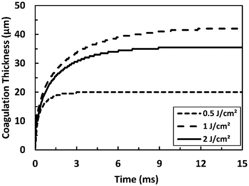
Figure 9. Predicted coagulation thickness as a function of the pulse fluence as a result of irradiation with Er:YAG laser pulse at several selected pulse durations (50, 500, and 1000 µs). The total simulation time is 15 ms.

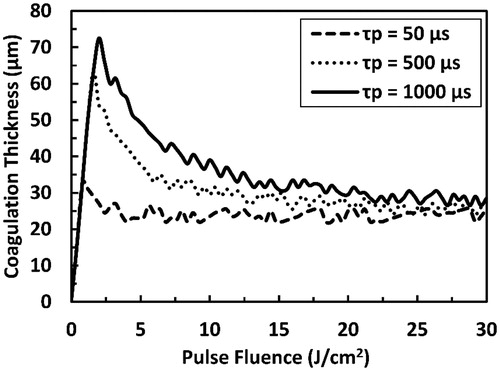
Figure 10. Predicted coagulation thickness as a function of pulse duration as a result of irradiation with ER:YAG laser pulse at several selected pulse fluences. F_th refers to the pulse fluence that is equal to the ablation threshold at each pulse duration and the dashed line connects the points where the transition from sub-ablative to ablative conditions occurs. The total simulation time is 15 ms.

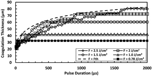
Figure 11. Predicted maximum coagulation thickness and ablation threshold at high strain-rate in comparison with those predicted at quasi-static loading for Er:YAG laser at pulse durations ranging from 10 µs to 2000 µs.

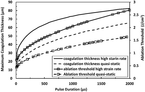
Figure 12. Predicted ablation efficiency as a function of both pulse duration and pulse fluence of a single Er:YAG laser pulse at (a) high strain-rate loading and at (b) quasi-static loading. Ablation efficency is the ratio between tissue-ablated mass and delivered laser energy.

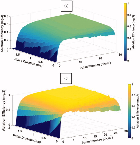
Table 2. Comparison between model predictions and experimental observations in terms of pulsed laser tissue ablation outcomes’ values and trends.

Outcome parameter’s value or trend	Model prediction	Experimental observation
Specific energy of ablation (Eab)	1.76 J mm^−3	1.5–1.75 J mm^−3 [51,52]
Surface temperature	470^oC	400–550 °C [53]
Maximum coagulation depth	90 µm	105 ± 25 µm and 75 ± 40 µm [9,54]
Coagulation versus pulse fluence and duration for the ablative modality	Asymptotically decrease with increasing pulse fluence and decreasing pulse duration	Asymptotically decrease with increased absorption coefficient, which has a similar effect as increasing pulse fluence or decreasing pulse duration when ablation is at work [9]
Minimum coagulation depth for the ablative modality	22–28 µm	16 ± 9 µm [9]
Effect of mechanical properties on ablation efficiency	Decreased in ablation efficiency with increased ultimate tensile strength and stiffness	Earlier, more rapid, and larger ablation for weaker tissues [34,49,55]
Ablation efficiency versus pulse fluence	Ablation efficiency increases and then saturates with increased pulse fluence	Saturation in ablation efficiency with increased pulse fluence [54]

Duck FA. Physical properties of tissues: a comprehensive reference book. Cambridge: Academic Press; 2013.

 Google Scholar

Venugopalan V, Nishioka N, Mikic B. The effect of laser parameters on the zone of thermal injury produced by laser ablation of biological tissue. J Biomech Eng. 1994;116:62–70.

 PubMed Web of Science ®Google Scholar

Walsh JT Jr, Deutsch TF. Pulsed CO2 laser tissue ablation: measurement of the ablation rate. Lasers Surg Med. 1988;8:264–275.

 PubMed Web of Science ®Google Scholar

Hibst R, Kaufmann R. Effects of laser parameters on pulsed Er-YAG laser skin ablation. Laser Med Sci. 1991;6:391–397.

 Google Scholar

Walsh JT Jr, Deutsch TF. Er: YAG laser ablation of tissue: measurement of ablation rates. Lasers Surg Med. 1989;9:327–337.

 PubMed Web of Science ®Google Scholar

Harris DM, Fried D, Reinisch L, et al. Eyelid resurfacing. Lasers Surg Med. 1999;25:107–122.

 PubMed Web of Science ®Google Scholar

Evers M, Ha L, Casper M, et al. Assessment of skin lesions produced by focused, tunable, mid‐infrared chalcogenide laser radiation. Lasers Surg Med. 2018;50:961–972.

 PubMed Web of Science ®Google Scholar

Hohenleutner U, Hohenleutner S, Bäumler W, et al. Fast and effective skin ablation with an Er: YAG laser: determination of ablation rates and thermal damage zones. Lasers Surg Med. 1997;20:242–247.

 PubMed Web of Science ®Google Scholar

Walsh JT, Deutsch TF. Pulsed CO/sub 2/laser ablation of tissue: effect of mechanical properties. IEEE Trans Biomed Eng. 1989;36:1195–1201.

 PubMed Web of Science ®Google Scholar

Apitz I, Vogel A. Material ejection in nanosecond Er: YAG laser ablation of water, liver, and skin. Appl Phys A. 2005;81:329–338.

 Web of Science ®Google Scholar

Apitz I, Vogel A. Material ejection in Q-switched Er: YAG laser ablation of water, liver, and skin. In Laser-Tissue Interaction XIV. International Society for Optics and Photonics; Vol. 4961. 2003. p. 48–60.

 Google Scholar