Feasibility and relevance of discrete vasculature modeling in routine hyperthermia treatment planning

Figures & data

Figure 1. Left: vessels skeleton and right: skeleton and connectivity. In this example, green points are starting points, red points are end points and purple points are bifurcations. The color of the squares around the points indicates that the point belongs to a separate tract of the vasculature.

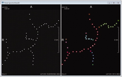
Table 1. EM and thermal simulation properties of tissues.

Tissue	εr	σ	ρ	c	k	Q	w
Internal air	1.00	0.0	1.2	–	–	–	–
Bone	13.07	0.09	1908	1313	0.32	0.15	10
Brainstem	55.11	1.05	1045.5	3630	0.51	11.4	558.6
Cartilage	45.14	0.60	1099.5	3568	0.49	0.54	35
Cerebellum	55.11	1.05	1045.5	3696	0.55	15.5	763.3
Cerebrum	56.81	0.75	1044.5	3653	0.51	15.7	770
CSF	70.63	2.26	1007	4096	0.57	0.0	763.3
Fat	11.59	0.08	911	2348	0.50	0.51	255
Grey matter	41.66	0.45	1041	3696	0.55	15.54	764
Lens	37.29	0.38	1075.5	3133	0.43	–	–
Lung	23.58	0.38	394	–	–	–	–
Muscle	56.87	0.80	1090.4	3421	0.4	0.96	442.8
Myelum	35.04	0.46	1075	3630	0.51	2.48	160.3
Optical nerve	35.04	0.46	1075	3613	0.49	2.48	160.3
Sclera	57.37	1.01	1032	4200	0.58	5.89	380
Thyroid gland	61.33	0.89	1050	3609	0.52	87.1	5624.3
Tumor	59.00	0.89	1050	3950	1.5	–	848
Vitreous humor	69.00	1.53	1004.5	4047	0.59	–	–
White matter	56.81	0.75	1044.5	3583	0.48	4.32	212

ε_r: relative permittivity; σ: conductivity (S/m); ρ: density (kg/m³); c: specific heat capacity (J/kg/°C); k: thermal conductivity (W/m/°C); Q: metabolic heat generation rate (W/kg); w: perfusion rate (mL/min/kg).

Figure 2. An example result of the graph-cut vessel segmentation algorithm. Pre-processed coronal slice of the MRA image of a patient with vessels segmentation color overlay in purple (left), and the skeletonization of the arterial vessel tree (right).

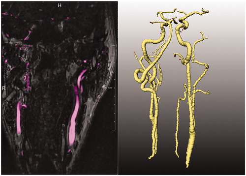
Figure 3. Maximum temperatures in the healthy tissue reached in PBHE + DIVA models with the same input powers as in PBHE models. The maximum temperature in the healthy tissue was 44 °C in the PBHE model.

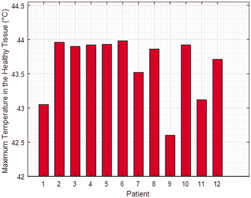
Figure 4. Differences in HTP quality parameters in the CTV (a) ΔT90 (|ΔT90avg| = 0.16 °C), (b) ΔT50 (|ΔT50avg| = 0.30 °C) and (c) ΔT20 (|ΔT20avg| = 0.33 °C). ‘*’ next to the patient number denotes a target volume that includes a part of the vessel tree.

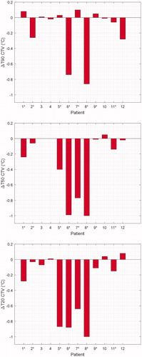
Figure 5. Example temperature distribution maps overlaid on CT images for PBHE (left), and DIVA (right).

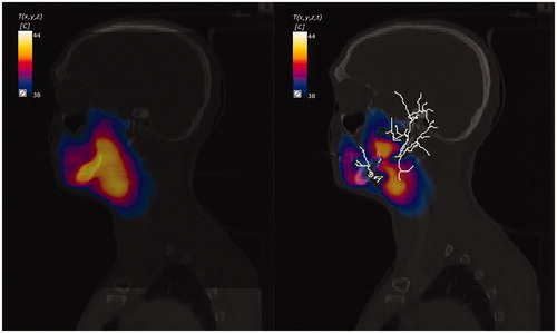
Figure 6. Principal verification benchmark: a coaxial setup involving a straight vessel inside a tissue cylinder.

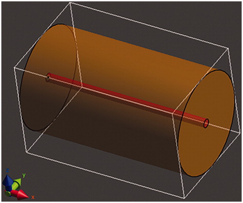
Table 2. Basic model parameters (in accordance with Table 1 in [24]).

Tissue conductivity	0.6 W·m^–1·K^–1
Tissue specific heat	4000 J·kg^–1·K^–1
Tissue density	1000 kg·m^–3
Tissue radius	0.003 m
Tissue length	0.01 m
Vessel radius	0.00025 m
Vessel length	0.01 m
Blood velocity	0.025 m·s^–1
Tissue initial temperature	1 °C
Inflow blood temperature	0 °C
Bucket density	5000
Number of grid voxels	31 × 31 × 50

Figure 7. (a) Theoretical and simulated temperature along the vessel for different bucket densities. Theoretical and simulated L_eq for a bucket density of (b) 5000, (c) 2500 and (d) 1250.

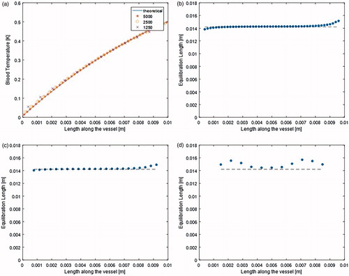
Figure 8. L_eq as a function of the vessel radius.

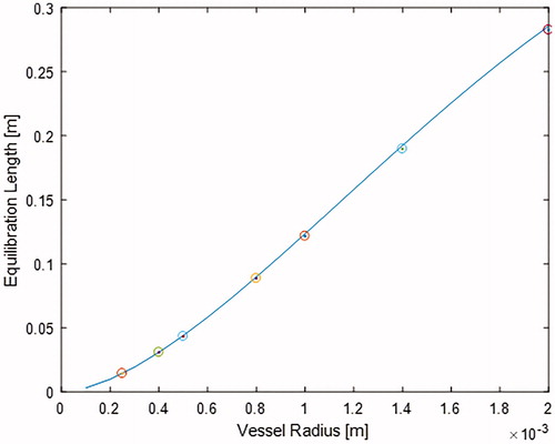
Figure 9. Temperature profile along three connected vessel segments (computed and theoretical; left) and L_eq (right).

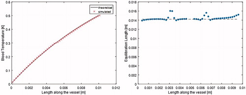
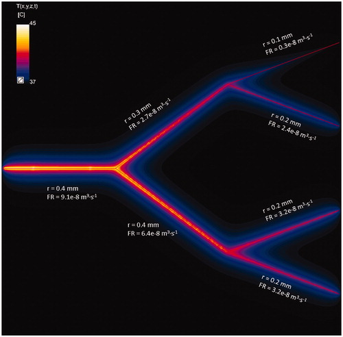
Figure 10. DIVA benchmark illustrating branching with symmetric and asymmetric flow-rate division. Red straight lines are indicating the vessel centerlines.

Kotte A, van Leeuwen G, de Bree J, et al. A description of discrete vessel segments in thermal modelling of tissues. Phys Med Biol. 1996;41:865–884.

 PubMed Web of Science ®Google Scholar