Figures & data
Figure 1. (a) Measured bandwidth of the RMV-710B transducer and (b) the frequency spectrum of a typical RF echo line through the gel phantom.
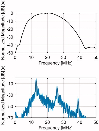
Figure 2. Schematic of the experimental setup. The side view of the setup shows that the hot needle is placed laterally 2 mm away from the imaging plane of the transducer and the tip of the thermocouple is placed within the imaging plane (2 mm away from the heating needle). The temperature at the thermocouple location changed from 26 °C to 46 °C.
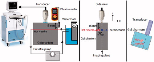
Figure 3. B-mode images of (left) tissue mimicking gel phantom and (right) ex vivo bovine muscle tissue. The temperatures measured by the inserted thermocouple were 31, 38, 42 and 46 °C at the center of heated region.
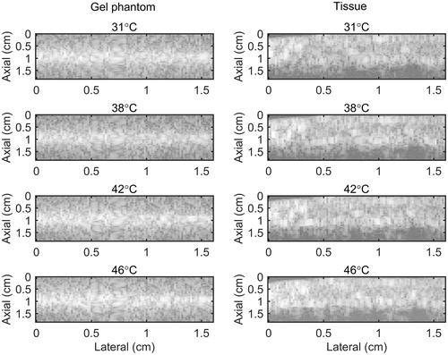
Figure 4. 2 D maps of CBE1 (left), CBE2 (middle), and CBE3 (right) in tissue mimicking gel phantom while the temperature was cooling down from 46 °C to 26 °C and no vibration was present in the phantom. The temperatures measured by the inserted thermocouple were 31, 38, 42 and 46 °C at the center of heated region. The color bars represent percentage change in backscattered energy. The horizontal rectangles are the regions of interest for calculating the CNR and SNR.
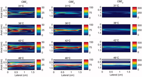
Figure 5. 2 D maps of CBE1 (left), CBE2 (middle), and CBE3 (right) in tissue mimicking gel phantom while the temperature was elevated from 26 to 46 °C with the presence of vibration in the phantom. The temperatures measured by the inserted thermocouple were 31, 38, 42 and 46 °C at the center of heated region. The color bars represent percentage change in backscattered energy. The heated region is along the arrow in the lower right panel.
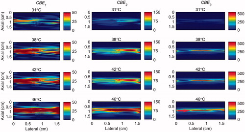
Figure 6. 2 D gradient maps in tissue mimicking gel phantom obtained using the conventional echo-shift technique without (left) and with (right) presence of vibration in the phantom. The temperatures measured by the inserted thermocouple were 31, 38, 42 and 46 °C at the center of heated region. The color bars represent the axial gradient of the cumulative time shifts in units of s/m. The horizontal rectangles are the regions of interest for calculating the CNR and SNR.
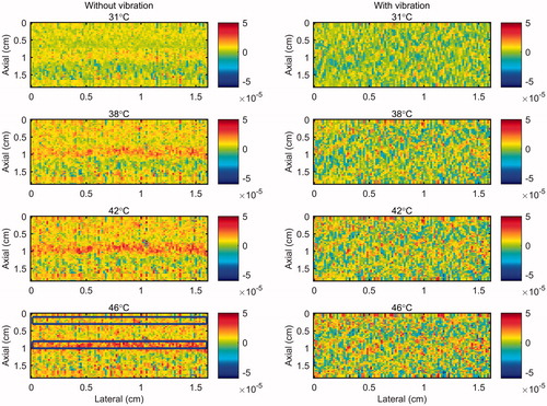
Table 1. The mean and the standard deviation of calculated SNR and CNR values for CBE and gradient maps with and without the presence of vibration in the gel phantom and tissue samples.
Figure 7. 2 D maps of CBE1 (left), CBE2 (middle), and CBE3 (right) in ex vivo bovine muscle tissue while the temperature was cooling down from 46 °C to 26 °C and no vibration was present in the tissue. The temperatures measured by the inserted thermocouple were 31, 38, 42 and 46 °C at the center of heated region. The color bars represent percentage change in backscattered energy. The horizontal rectangles are the regions of interest for calculating the CNR and SNR.
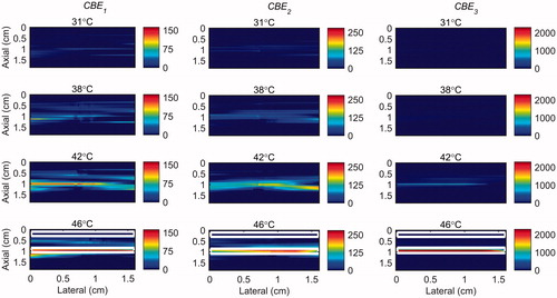
Figure 8. 2 D maps of CBE1 (left), CBE2 (middle), and CBE3 (right) in ex vivo bovine muscle tissue while the temperature was elevated from 26 to 46 °C with the presence of vibration in the tissue. The temperatures measured by the inserted thermocouple were 31, 38, 42 and 46 °C at the center of heated region. The color bars represent percentage change in backscattered energy. The heated region is along the arrow in the lower right panel.
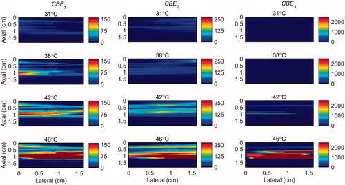
Figure 9. 2 D gradient maps in ex vivo bovine muscle tissue obtained using the conventional echo-shift technique without (left) and with (right) presence of vibration in the tissue. The temperatures measured by the inserted thermocouple were 31, 38, 42 and 46 °C at the center of heated region. The color bars represent the axial gradient of the cumulative time shifts in units of s/m. The horizontal rectangles are the regions of interest for calculating the CNR and SNR.

Figure 10. The mean and standard deviation of CBE1, CBE2 and CBE3 in (a) tissue-mimicking gel phantoms and (b) ex vivo bovine muscle tissues as a function of temperature. The error bars represent the standard deviation in five trials with two samples of tissue and gel phantoms.
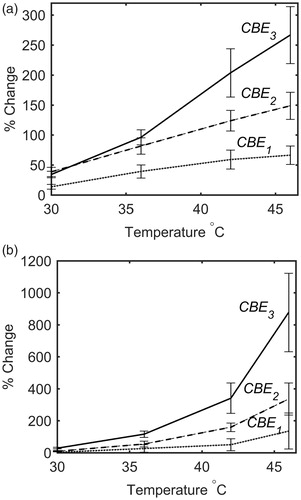
Table 2. The standard deviation of CBE1, CBE2 and CBE3 in (left) one and (right) five trials with two tissue-mimicking gel phantoms of the same composition at three temperatures.
Table 3. The standard deviation of CBE1, CBE2 and CBE3 in (left) one and (right) five trials with two different ex vivo bovine muscle tissues at three temperatures.
Figure 11. The mean and standard error of CBE1, CBE2 and CBE3 in ex vivo bovine muscle tissues as a function of temperature. The error bars represent the standard error in five trials. The red and blue lines represent the lower and upper temperature band, respectively.
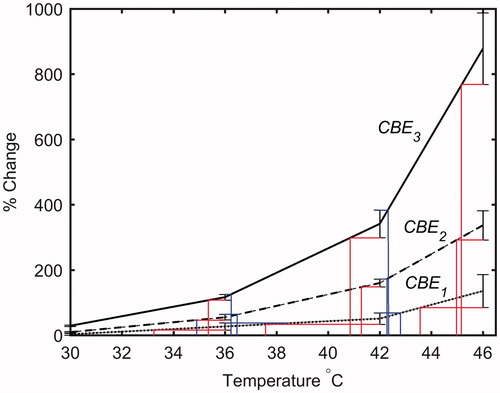
Table 4. The temperature range corresponding to mean minus SE and mean plus SE of CBE1, CBE2 and CBE3 in ex vivo bovine muscle tissues at three measured temperatures.
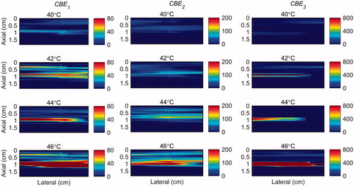
Figure 12. 2 D maps of CBE1 (left), CBE2 (middle), and CBE3 (right) in tissue mimicking gel phantom while the temperature was elevated from 38 to 46 °C. The temperatures measured by the inserted thermocouple were 40, 42, 44 and 46 °C at the center of heated region. The color bars represent percentage change in backscattered energy (with a 38 °C baseline).
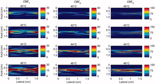
Figure 13. 2 D maps of CBE1 (left), CBE2 (middle), and CBE3 (right) in ex vivo bovine muscle tissue while the temperature was elevated from 38 to 46 °C. The temperatures measured by the inserted thermocouple were 40, 42, 44 and 46 °C at the center of heated region. The color bars represent percentage change in backscattered energy (with a 38 °C baseline).