
Figures & data
Figure 1. CT-guided implantation process. (A) Self-made positioning fence. (B) Self-made positioning fence (white arrow) displayed on a CT image. (C) The axial scan showed that the puncture needle had punctured into the lower pole of the kidney. (D) Coronal reconstruction indicates the full length of the needle and a more intuitive display of the needle tip position.
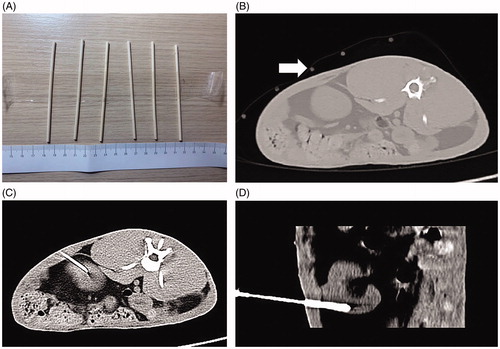
Figure 2. MR-guided puncture of renal tumors. (A) Preoperative surface localization by a vitamin E capsule (white arrow). (B) The 3D-VIBE-T1WI axial scan revealed that the needle antenna was punctured into the kidney, but its relationship with the lesion could not be distinguished. FS-TSE-T2WI oblique-coronal (C) and oblique-axial (D) scans obviously indicated that the needle antenna was positioned within the renal tumor.
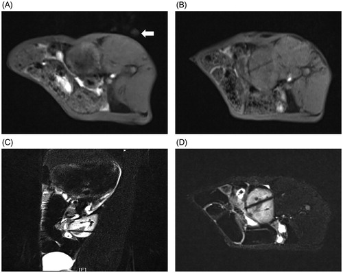
Figure 3. Gross pathological examination before MWA. (A) The tumor was located in the lower pole of the kidney (arrow). (B) The tumor was white in color on the cut surface (arrow).
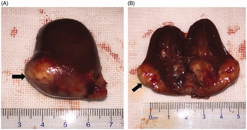
Figure 4. Histopathological findings for the VX2 tumor in HE staining. (A) The tumor cells were nest-arranged and invaded the normal renal parenchyma. (B) Residual glomerulus (black arrow) was destroyed partially by tumor cells (white arrow). (C) Coagulation necrosis was found in the center of the cancer nest. (D) Pathological mitotic figures of tumor cells could be seen (black arrow). (E) Tumor giant cell was found (black arrows).
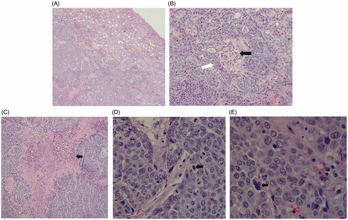
Figure 5. MRI findings of the VX2 tumors in the left kidney. (A) The 1.5-Tesla 3D-volumetric interpolated breath-hold examination T1-weighted imaging analysis showed a heterogeneous iso-low signal. (B) The VX2 tumor showed a circular low signal, as indicated by 1.5-Tesla fat suppression turbo spin-echo T2-weighted imaging analysis. (C) Diffusion-weighted imaging analysis showed that VX2 tumors exhibited a high signal. 3D-VIBE-T1WI (D) and FS-TSE-T2WI coronal (E) scans revealed that the tumor was located in the lower pole of the left kidney.
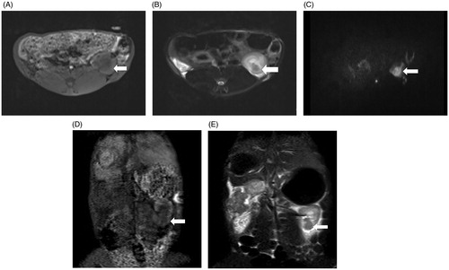
Figure 6. Explanation of the nephrometry scoring system. (A) R (radius): tumors ≤4 cm are assigned 1 point, those >4 but <7 cm are assigned 2 points, and those >7 cm are assigned 3 points. (B) E (exophytic/endophytic): tumors that are 50% or more exophytic are assigned 1 point, tumors that are less than 50% exophytic are assigned 2 points, those that are completely inside the renal cortex are assigned 3 points. (C) N (nearness): Tumors that are ≥7 mm far from the collecting system or sinus are assigned 1 point, tumors that are >4 but <7 mm far from the collecting system or sinus are assigned 2 points, and those <7 mm far are assigned 3 points. (D) A (anterior): If the tumor is located on the ventral surface, the suffix “a” is assigned; if it is located on the dorsal surface, the suffix “p” is assigned; and if it is not possible to clearly identify the location of tumor, the suffix “x” is assigned. (E) L (location): If tumors are entirely located above or below the polar lines, then 1 point is assigned, tumors that exceed the polar lines but within <50% are assigned 2 points, and those that exceed >50% or entirely between the upper polar line and lower polar line are assigned 3 points.
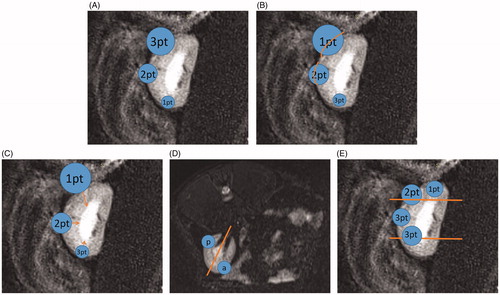
Figure 7. Flow chart of the study.
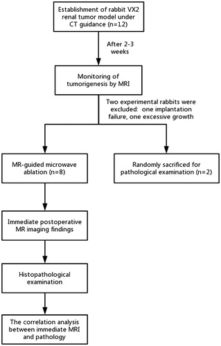
Table 1. Score assignment for the 10 successfully implanted tumors.
Figure 8. Immediate efficacy of postoperative MR-guided MWA. (A). 3D-VIBE-T1WI sequence typically indicated a “target sign.” Notably, the original tumor in the center of the ablation zone showed low signal intensity (thin arrow), and a high signal intensity completely surrounded the primary tumor with a clear boundary in the ablation zone (thick arrow). (B) On FS-TSE-T2WI, the signal intensity of the primary tumor was lower than that before (thin arrow), while the lesion with an unclear boundary was completely covered with a low signal intensity in the ablation zone (thick arrow). 3D-VIBE-T1WI (C) and FS-TSE-T2WI (D) oblique-coronal scans clearly revealed the location of the ablation zone.
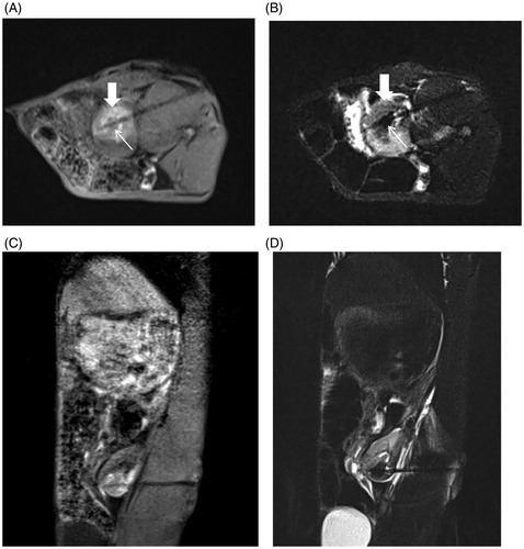
Figure 9. Gross pathological examination after ablation. (A) Ablated tumor was located in the lower pole of the left kidney (black arrow). (B) The ablative change showed a black carbonized needle track along the microwave antenna path (black triangle) with yellow-white coagulation necrosis in the center of the original tumor (black arrow). Another gray yellow coagulation necrosis area was also found besides the tumor (white arrow). Moreover, a dark red band congestion and edema area was detected around the ablative lesion.
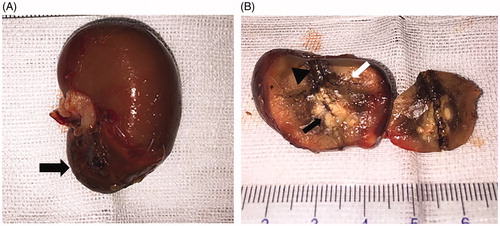
Figure 10. Histopathological findings of the renal ablation zone determined by HE staining. (A) The ablation zone was divided into three different zones: coagulation necrosis of tumor nests ①, coagulation necrosis of normal renal parenchyma ②, and congestion and edema band③. (B) Pink exudate was found in the coagulation necrosis area of normal renal parenchyma (black arrow). (C) Markedly dilated spaces between the cords of neoplastic cells (circles). (D) Coagulation necrosis area of the tumor showed a residual cell outline with karyolysis (black arrow). (E) Tubular dilatation was found in the tumor coagulation necrosis area (black triangle). (F) Infiltration of lymphocytes (black arrow) in the hemorrhagic zone (A, ×4; B, E, and F, ×20; C and D, ×40 magnification).
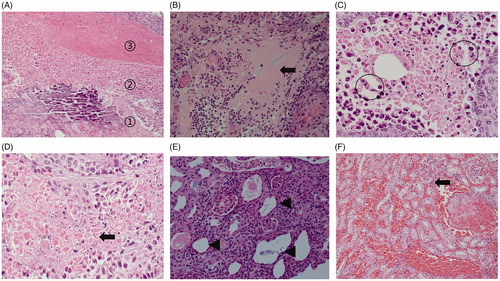
Table 2. Comparison of the volume of tumors between MR images and tissue specimens.
Table 3. Comparison of the ablation zone size between MR images and tissue specimens.