T2 mapping as a predictor of nonperfused volume in MRgFUS treatment of desmoid tumors

Figures & data

Figure 1. Positioning of patient 1 is shown via axial (a), coronal (b), and sagittal (c) view. These localizer images additionally show the transducer, gel pad, and cooling water bag.

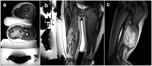
Table 1. Overview of sonication and acquisition data sorted by patient.

	# of MRgFUS treatment sonications	Energy range of sonications (J)	Temperature range of sonications (°C)	# of T2 map acquisitions	T2 map type
Patient 1	69	1745–2268	49–77	6	Double-echo FSE
Patient 2	70	1284–1556	50–96	4	Double-echo FSE
Patient 3	79	1699–7897	38–83	6	Multiecho FSE
Patient 4	78	1536–6591	37–80	4	Multiecho FSE
Patient 5	76	1751–6882	40–94	4	Multiecho FSE

Figure 2. Sagittal T2 maps of one slice of the treatment region of patient 1. (a) Demonstrates the tissue before sonication treatment. (b–e) demonstrate increased T2 value over the course of the treatment duration—4 h. (f) Shows the T2 value approximately 20 min after treatment has ended. 2(right) is a quantification of this signal at the given ROI over time where the dotted arrowhead represents the final sonication treatment, just before point ‘e’. T2 maps were generated in MatLab.

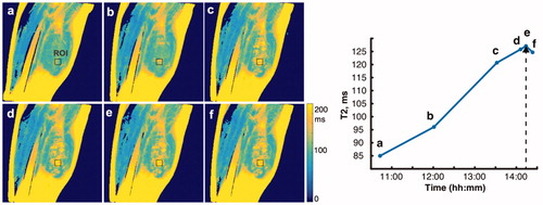
Figure 3. Comparison of a sagittal T2 map (a) with post-treatment postcontrast image (b) of same location for patient 1. The nonperfused volume (NPV) appears hyperintense on T2 maps (example given by ROI box). Consequently, the red arrows identify gaps in the NPV, which correspond to high enhancement in the postcontrast images.

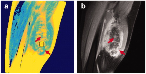
Figure 4. Axial T2 maps (a–c) of one slice of the treatment region of patient 2. (a) Demonstrates the tissue before sonication treatment. (b and c) Demonstrate increased T2 value over the course of the treatment duration. (d) A post-contrast image of same location. Patient was repositioned, but the arrows indicate the ROI. T2 maps were generated in MatLab.

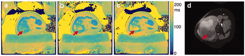
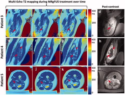
Figure 5. Multi-slice T2 maps were generated (one slice shown). T2 maps for three additional patients are shown pre-sonication (first column: a, e, i), mid-sonication (second column: b, f, j) and end-sonication (final column: c, g, k). This set of final T2 maps is intended for comparison to d, h, l which demonstrate the corresponding postcontrast images.