Figures & data
Table 1. Phantom ingredients.
Figure 1. Schematic of through-transmission experimental setup. The signal generator sends a five-cycle burst to the transmit transducer. The generated acoustic wave travels through the phantom or a water-only reference sample, and the oscilloscope records the remaining transmitted signal after amplification. The use of a broadband transmit transducer (V314, Panametrics-NDT, Waltham, MA, USA) enables the acoustic properties to be measured at transmit carrier frequencies of 0.6, 1.0, 1.8, and 3.0 MHz.
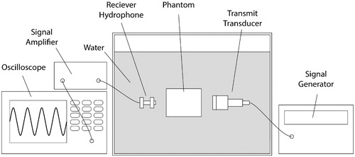
Figure 2. Schematic of the setup used to perform repeatable ultrasound B-mode imaging and shear-wave speed measurements.
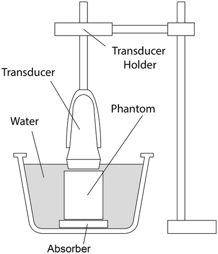
Figure 3. Measured MR (a and b) and acoustic properties (c and d) for nine different psyllium husk concentrations. Error bars in T1, T2, and T2* relaxation rates (a and b) denote the measurement standard deviation over the 15 × 15 pixel ROI from which the average values were calculated. Error bars in the acoustic property measurements (c and d) denote the standard deviation of the three repeated measurements.
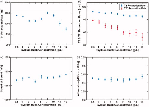
Figure 4. US B-mode images and GRE MR magnitude images (TE = 25.4 ms) are depicted for five different psyllium husk concentrations. The schematic line drawings on the left depict the orientation of the imaging planes for the US and MR images relative to the phantom cylinder. The rubber cork stopper used to seal the phantom likely caused the enhanced or decreased image intensity seen on the left side of the MR magnitude images.
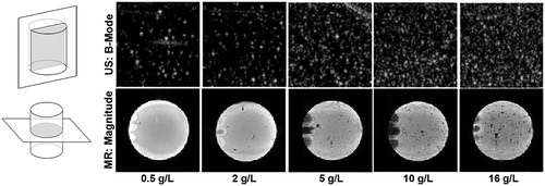
Figure 5. Measured mean shear-wave speed as a function of psyllium husk concentration is shown in (a). US shear-wave speed maps at three different phantom temperatures for the 10 g/L phantom are shown in (b–d).
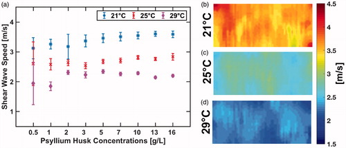
Figure 6. Measured shear-wave speed as a function of phantom age for 10-g/L psyllium husk phantom.
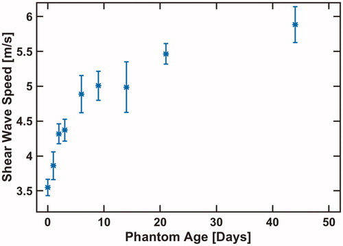
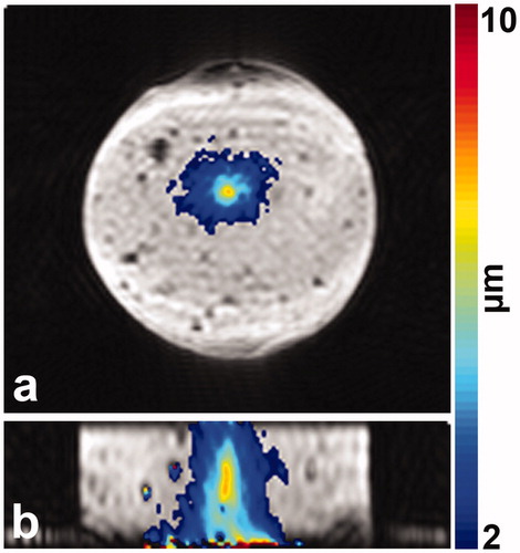
Figure 7. 3 D MR-ARFI displacement maps in coronal (a) and sagittal (b) plane are depicted as a color overlay on the segmented EPI magnitude image.