Mathematical modeling of the thermal effects of irreversible electroporation for in vitro, in vivo, and clinical use: a systematic review

Figures & data

Figure 1. Flow diagram of the study selection.

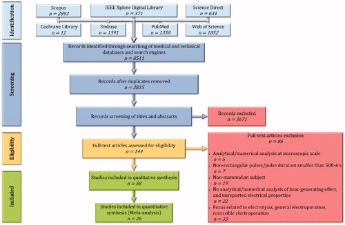
Figure 2. Overview of IRE pulses, with V_P [V] as the electric potential (the voltage) of the pulses, t_P [s] as the duration of a single pulse, n_P as the pulse number, N_P as the total number of pulses, τ_P [s] as the duration between two pulses, and f_P [Hz] as the pulse frequency.

Figure 3. Examples of applied boundary conditions for the calculations of the electric potential distribution with arrow representing electric-current flow through the outer surface of the model (I_BOS [A]). The red and the blue circles represent BEM with the electrodes given in the color gray, and black lines represent the BOS of the model. (A) shows Dirichlet boundary conditions at BEM and BOS, and (B) shows Dirichlet boundary conditions at BEM, and Neumann boundary conditions at BOS if I_BOS = 0 A or Robin boundary conditions if I_BOS is limited.

Figure 4. Examples of applied boundary conditions for the calculations of the temperature distribution. The brown circles represent BEM with the electrodes given in the color gray, and black lines represent the BOS of the model. Arrows represent heat flux vector that is normal to the BEM (q_BEM [W⋅m⁻²]) and the BOS (q_BOS [W⋅m⁻²]). At both BEM and BOS (A) shows Dirichlet boundary conditions, and (B) shows Neumann boundary conditions if q_BEM = 0 W⋅m⁻² and q_BOS = 0 W⋅m⁻², or Robin boundary conditions if q_BEM and q_BOS are limited.

Figure 5. (A) Assumed model that includes infinite electrode plates to calculate the temperature increase during IRE. The electrodes are presented as gray rectangles with infinite length and IRE-TR as a yellow rectangle. The black triangle represents a possible location in the model with maximum temperature increase. (B) An example of a temperature increase profile based on Equation 7(7) $$\mathrm{\Delta }\mathrm{T}=\frac{\mathit{J}·\mathit{E}·{\mathrm{t}}_{\mathrm{P}}·{\mathrm{f}}_{\mathrm{P}}}{\mathrm{\rho }{\mathrm{c}}_{\mathrm{p}}}\mathrm{\Delta }\mathrm{t}$$(7) , which is divided in normothermia (from t_init to t_MH), moderate hyperthermia (MH; from t_MH to t_TA), and thermal ablation (TA; from t_TA to t_end).

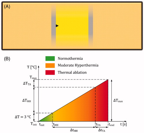
Figure 6. Examples of electrode configurations applied in studies to calculate the electric-field distribution, with the colors gray and brown as metallic and insulation parts, respectively. These configurations represent: (A) spherical electrodes, (B) needle and surface electrodes, (C) circular plate electrode enclosed by a ring electrode, (D, E) plate electrodes, (F) endovascular electrodes; contralateral electrodes have the same electric potential, (G) needle electrodes, (H) bipolar needle electrode; contralateral electrodes have different electric potential. In each configuration, the distances d [m] and D [m] were defined for the calculation of the energy density. Several studies assumed the needle and bipolar electrodes to be cylinders in 3D models. Other studies assumed the needle and spherical electrodes to be circles in 2D models.

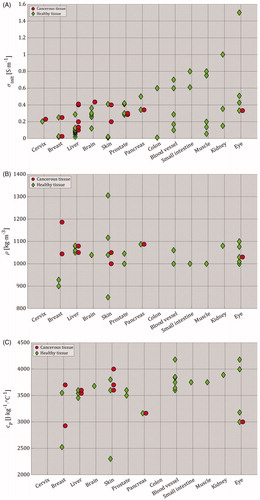
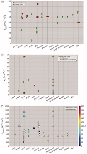
Table 1. Summary of organ-dependent electrical and thermal characteristics for cancerous and healthy tissues (see Supplementary Appendix 6 – Table A6.2).

Electrical and thermal properties	Cancerous tissue	Healthy tissue
Initial electric conductivity (σinit [S⋅m^−1])	[0.025, 0.435]^a	[0.01, 1]^b
Mass density (ρ [kg⋅m^−3])	[1000, 1186]	[850, 1305]
Specific heat capacity (cp [J⋅kg^−1⋅°C^−1])	[2926, 4000]	[2300, 4180]
Initial thermal conductivity (kinit [W⋅m^−1⋅°C^−1])	[0.4, 0.75]	[0.0565, 0.565]
Blood perfusion (wb [kg⋅m^−3⋅s^−1])	[1, 19.08]^c	[0.5, 19.08]^c
Electric-field threshold of irreversible electroporation (EIRE(th) [V⋅m^−1])	[500 × 10^2, 1700 × 10^2]	[213 × 10^2, 1750 × 10^2]

Please note that the brackets ([min, max]) indicate the range between and including the minimum and maximal selected values. Also note that the rare instances of values that exceeded 1 S⋅m⁻¹ for the initial electrical conductivity (σ_init [S⋅m⁻¹]) were 1.5 S⋅m⁻¹ for aqueous and vitreous in the eye [44], and 2.31 S⋅m⁻¹ for cancerous breast tissue [28]. In case of blood perfusion (w_b [kg⋅m⁻³⋅s⁻¹]), the value that exceeded 20 kg⋅m⁻³⋅s⁻¹ was 212 kg⋅m⁻³⋅s⁻¹ for both healthy and cancerous pancreas tissues [70]. If w_b could not be extracted nor calculated due to the absence of blood density (ρ_b [kg⋅m⁻³]), then w_b was calculated by assuming ρ_b = 1060 kg⋅m⁻³.

^a2.31 S⋅m⁻¹ was reported as the maximum value for cancerous breast tissue [28].

^b1.5 S⋅m⁻¹ was reported as the maximum value for aqueous and vitreous in the eye [44].

^c212 kg⋅m⁻³⋅s⁻¹ was reported as the maximum value for both healthy and cancerous pancreas tissues [70].

Figure 8. (A) The study characteristics ‘Tissue type’, ‘ΔT_max’, ‘σ_init’, ‘Electrode type’, and ‘u’ were plotted as function of ‘Pulse voltage (V_P [V])’ and ‘Total pulsing time (t_P ⋅ N_P [s])’ in logarithmic scale. For a proper clarification of the data points, an extended version can be found in Supplementary Appendix 4 Figure A4.1. The range of ΔT_max was 0.27 ≤ ΔT_max [°C] ≤ 135, which was represented by the linearly scaled red-yellow color bar with the range 0 ≤ ΔT_max [°C] ≤ 40. The ΔT_max values that exceeded 40 °C were 50 °C at (750 V, 9 × 10⁻³ s) [34], 55 °C at (1500 V, 1 × 10⁻² s) [64], 85 °C at (2000 V, 3 × 10⁻⁴ s) [55], and 135 °C at (2000 V, 3 × 10⁻⁴ s) [55]. Furthermore, the range of u was 1.19 × 10⁵ ≤ u [J⋅m⁻³] ≤ 11.42 × 10⁸, which was represented by the linearly scaled blue-magenta color bar with the range 0 ≤ u [J⋅m⁻³] ≤ 10 × 10⁸. The u values that exceeded 10 × 10⁸ J⋅m⁻³ were two times the value 11.42 × 10⁸ J⋅m⁻³ at (2000 V, 9 × 10⁻³ s) [44]. (B) Here, we only plotted the data that was obtained from the pulse parameters which were applied in the experiments. The range of ΔT_max was 1 ≤ ΔT_max [°C] ≤ 39, and the range of the energy density was 2.92 × 10⁶ ≤ u [J⋅m⁻³] ≤ 8.22 × 10⁸. (C) is similar to (B), with the exception of having ‘Total treatment time (N_P ⋅ f_P⁻¹ [s])’ in logarithmic scale instead of ‘Total pulsing time’. Please note the change in Y-axis in (C) in comparison to (B), and that the electrical conductivity is the conductivity before the treatment.

Figure 9. Linear regression plots of R_3ΔT13 and R_ΔT13 data points as function of S_E-IRE(th). For a proper clarification of the data points, an extended version can be found in Supplementary Appendix 4 Figure A4.2. The ΔT_max and the u ranges were 1.9 ≤ ΔT_max [°C] ≤ 39, and 0.29×10⁷ ≤ u [J⋅m⁻³] ≤ 8.44 × 10⁷. Please note that the scale of the color bar of the energy density in this figure is different than the scales in Figure 8. In addition, the symbols at (4.83 × 10⁻⁵ m², 0.32%) and (4.83 × 10⁻⁵ m², 9.19%) have a gray background since the ΔT_max was not reported.

Figure 10. (A) Linear regression plot of ΔT_max data points as function of the energy density. (B) Linear regression plots of R_3ΔT13 and R_ΔT13 data points as function of the energy density. Please note the change in X-axis in (B) in comparison to (A).

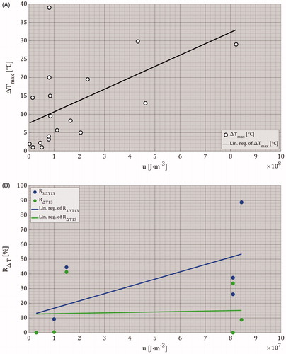
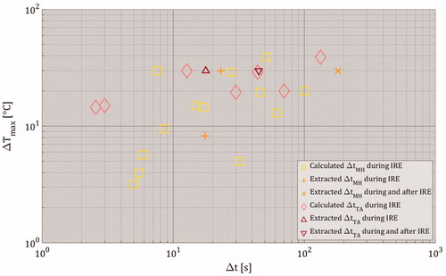
Figure 11. The estimated time durations for both mild hyperthermia and thermal ablation as function ΔT_max. The term ‘Extracted’ means that Δt_MH and Δt_TA values were directly provided by the included studies, while the term ‘Calculated’ signifies that Δt_MH and Δt_TA were calculated using the assumptions stated in the Subsection 3.2.2.3. Estimation of time durations of mild-hyperthermic and thermally ablative temperatures. Please note that Δt represents the duration of mild-hyperthermic effect (3 °C ≤ ΔT_max < 13 °C) and thermal ablative effect (ΔT_max ≥ 13 °C) of an included study. The ΔT_max only represents the maximal temperature increase obtained from the included study. Also, note that the value of Δt_MH was 0 s for ΔT_max < 3 °C and the value of Δt_TA was 0 s for ΔT_max < 13 °C.

Mandel Y, Rubinsky B. Treatment of uveal melanoma by nonthermal irreversible electroporation: electrical and bioheat finite element model of the human eye. J Heat Transf Trans ASME. 2012;134(11):111101.

 Web of Science ®Google Scholar

Daniels C, Rubinsky B. Electrical field and temperature model of nonthermal irreversible electroporation in heterogeneous tissues. J Biomech Eng Trans ASME. 2009;131(7):071006.

 PubMed Web of Science ®Google Scholar

Latouche EL, Sano MB, Lorenzo MF, et al. Irreversible electroporation for the ablation of pancreatic malignancies: a patient-specific methodology. J Surg Oncol. 2017;115(6):711–717.

 PubMed Web of Science ®Google Scholar

Maor E, Rubinsky B. Endovascular nonthermal irreversible electroporation: a finite element analysis. J Biomech Eng Trans ASME. 2010;132(3):031008.

 PubMed Web of Science ®Google Scholar

van Gemert MJC, Wagstaff PGK, de Bruin DM, et al. Irreversible electroporation: just another form of thermal therapy? Prostate. 2015;75(3):332–335.

 PubMed Web of Science ®Google Scholar

Kurata K, Nomura S, Takamatsu H. Three-dimensional analysis of irreversible electroporation: estimation of thermal and non-thermal damage. Int J Heat Mass Transf. 2014;72:66–74.

 Web of Science ®Google Scholar