Radiofrequency applicator concepts for thermal magnetic resonance of brain tumors at 297 MHz (7.0 Tesla)

Figures & data

Figure 1. Overview over all 10 RF applicator designs investigated in this work. In the center column, cross-sectional view of the RF arrays depicts the arrangement of the building blocks around the head and details about their position with respect to each other. The rightmost column shows the designs and their positioning for the small tumor model.

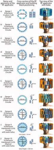
Table 1. Materials and dielectric parameters used for electromagnetic field simulations.

Model	Component	Material	σ (S/m)	ɛr	ρ (g/cm³)
Small tumor model	Tumor growth	Tumor	1.15	66.5	1025.5
	Duke	All tissues	IT’IS database
	Closed layer of CSF	Dura → CSF	2.22	72.8	1007
Large tumor model	Tumor growth	Tumor	1.15	66.5	1025.5
	Brain	40% WM + 60% GM	0.52	50.3	1043
	Brainstem	40% WM + 60% GM	0.52	50.3	1043
	Tissue	Fat	0.07	11.7	911
		Muscle	0.77	58.2	1090.4
	Skull	Bone	0.08	13.5	1908
	Eye	Vitreous humor	1.52	69.0	1004.5
	Optical nerve	Nerve	0.42	37.0	1075
	Chiasm
	Spinal cord
	Vessels	Blood	1.32	65.7	1049.8
	Cavities	Air	0	1	1
	Pituitary gland	Hypothalamus	0.85	62.5	1053
	Hypothalamus
Heavy water resonator (design 1)	Dielectric resonator	Heavy water (D2O)	0.02	81	1000
	Casing	Plexiglass (PMMA)	0.025	3.6	1180
	Antenna substrate	FR-4	0.025	4.3	1800
	Bow tie antenna	PEC
High permittivity resonator (designs 2–10)	Dielectric resonator	Ceramic slurry	0.2	200	6020
	Casing	Plexiglass (PMMA)	0.025	3.6	1180
	Antenna substrate	FR-4	0.025	4.3	1800
	Bow tie antenna	PEC
	Water bolus (designs 9 + 10)	Deionized water	0.016	81	1000

WM: white matter; GM: gray matter.

Parameters sources: tumor tissue [34]; body tissues [35]; D₂O, deionized water, ceramic slurry: bench measurement based on an open-end coaxial probe setup [36,37]; PMMA, FR-4: material datasheets.

Figure 2. (a) Schematic presentation of the workflow from the diagnostic MRI of the patient to the SAR_10g distribution as the hyperthermia treatment planning. (b) Details of the simulation and optimization process from the tumor models to the metrics to be evaluated to assess the RF array for hyperthermia treatment planning and magnetic resonance imaging performance.

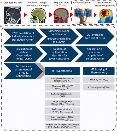
Table 2. Summary of all metrics assessing the performance of the RF-applicators, including the worst reflection and coupling coefficients (column 1, ‘Scattering’), the Hyperthermia Treatment Planning (HTP) results using the power optimization (column 2, ‘Power optimization’), the HTP results using the uniformity optimization (column 3, ‘Uniformity Optimization’) with # indicating the number of additive excitation phase and amplitude settings as well as the results of the B₁⁺ shimming (column 4, ‘MRI’) for the small tumor model (top half) and the large tumor model (bottom half).

	Scattering		Power optimization									Uniformity optimization									MRI
	Sii,max (dB)	Sij,max (dB)	#	SAR10g,max(TV) ($\frac{\mathrm{W}}{\mathrm{kg}}$)	SAF	TCSAR>Lim (%)	PHead (W)	PTumor (W)	PI ($\frac{\mathrm{W}}{\mathrm{kg}}$)	TC25% (%)	HTQ	#	SAR10g,max(TV) ($\frac{\mathrm{W}}{\mathrm{kg}}$)	SAF	TCSAR>Lim (%)	PHead (W)	PTumor (W)	PI ($\frac{\mathrm{W}}{\mathrm{kg}}$)	TC25% (%)	HTQ	B1^+ ($\frac{\text{μT}}{\sqrt{\mathrm{k}\mathrm{g}\cdot \mathrm{W}}}$)	COV (%)
Small tumor model
Design 1	–32.5	–12.5	2	46.7	2.8	36.0	74.2	1.5	47	100	1.00	2	43.8	2.4	18.9	81.2	1.4	20	100	1.04	0.25	21.7
Design 2	–89.5	–30	1	51.4	2.7	47.2	86.2	1.6	66	100	0.90	2	48.5	2.2	57.4	104.2	1.6	62	100	0.92	0.21	19.2
Design 3	–71.5	–19.5	1	53.9	3.6	65.3	70.9	1.7	126	100	0.84	2	53.1	3.1	77.2	85.8	1.8	127	100	0.84	0.14	16.4
Design 4	–91	–30.5	1	56.3	3.4	73.3	77.0	1.8	140	100	0.79	2	54.8	3.0	72.9	86.1	1.8	120	100	0.82	0.13	17.4
Design 5	–97	–28.5	2	59.0	4.6	65.5	55.1	1.8	178	100	0.81	2	57.4	3.5	66.9	75.9	1.8	135	100	0.84	0.08	14.3
Design 6	–110	–40.5	2	59.3	3.0	66.7	64.6	1.7	152	100	0.83	2	50.4	3.3	59.9	72.1	1.6	99	100	0.88	0.14	17.5
Design 7	–66	–20	2	57.1	4.6	73.0	47.6	1.5	191	100	0.77	2	51.9	3.5	69.9	70.1	1.7	125	100	0.85	0.02	11.0
Design 8	–67.5	–17.5	1	51.3	4.1	55.4	51.3	1.6	116	100	0.88	2	46.4	2.6	43.8	82.5	1.5	52	100	0.97	0.04	9.9
Design 9	–77.5	–29.5	1	55.8	6.2	70.6	38.5	1.8	244	100	0.83	1	53.0	5.1	65.2	44.2	1.7	178	100	0.87	0.08	24.1
Design 10	–73	–27.5	1	56.6	6.6	74.6	36.6	1.8	277	100	0.82	1	53.6	5.6	63.5	40.1	1.7	191	100	0.88	0.04	25.3
Large tumor model
Design 1	–62	–21.5	2	57.3	2.0	18.8	84.1	13.6	21	100	1.21	2	45.2	1.8	3.2	87.5	12.2	3	100	1.28	0.59	28.1
Design 2	–85.5	–30.5	2	73.4	2.0	37.2	104.5	16.6	55	100	0.97	2	48.1	2.0	4.6	73.4	11.6	4	100	1.11	0.05	25.1
Design 3	–88.5	–32.5	2	96.4	2.7	45.5	87.0	18.3	117	93	0.86	2	82.4	2.4	47.5	97.2	18.0	93	100	0.92	0.05	20.1
Design 4	–88.5	–32	1	94.8	2.9	43.0	74.7	18.0	120	86	0.85	2	80.9	2.6	45.8	84.4	18.1	95	100	0.91	0.09	19.7
Design 5	–109.5	–44	2	100.3	3.0	59.1	92.8	20.6	174	98	0.77	2	75.5	2.6	49.6	95.7	18.0	99	100	0.88	0.10	20.4
Design 6	–107	–40.5	1	108.3	3.5	55.6	72.7	20.6	210	84	0.79	2	91.3	3.0	46.7	76.5	18.7	128	100	0.85	0.07	17.7
Design 7	–64.5	–20.5	2	70.7	2.4	47.9	91.8	17.8	82	100	0.87	2	59.6	2.5	31.9	84.7	16.0	47	100	0.98	0.05	14.2
Design 8	–65.5	–17.5	2	85.6	3.0	50.2	72.4	19.2	131	100	0.84	2	85.4	3.5	43.7	60.4	18.1	131	100	0.89	0.04	14.8
Design 9	–63.5	–24.5	1	104.6	3.1	32.5	62.4	16.3	105	76	0.99	2	101.1	3.0	29.7	63.6	15.9	89	80	1.02	0.07	28.6
Design 10	–71.5	–21	1	79.9	3.8	46.3	55.6	18.9	141	93	0.91	3	69.5	3.0	29.9	60.5	16.9	63	100	1.06	0.07	30.5

The best results are highlighted in green and bold while the worst results are red and italic.

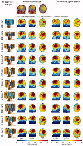
Figure 3. Top row: sagittal, coronal and axial section through the small tumor model. Left: description and front view of each design simulated together with the small tumor model; maximum intensity projection of the SAR_10g distribution after hyperthermia treatment planning for the power optimization (center) and the uniformity optimization (right).

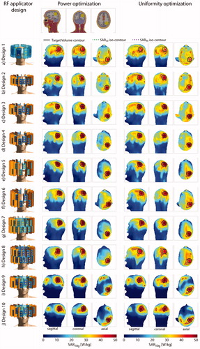
Figure 4. Qualitative comparison of the metrics used to assess HTP quality. The top row displays the results obtained for the small tumor model; the bottom row shows the results for the large tumor model. The results in the left column are obtained using the power optimization; the results of the uniformity optimization are in the right column. Blue lines highlight designs 9 and 10 equipped with a water bolus. All values are normalized to their respective intra-design, intra-optimizer maximum. Metrics labeled with a green font combine to the performance indicator. For better visualization so that higher values are always better, we plotted the reciprocal of the HTQ (1/HTQ = THQ). For the small tumor model, adding the water bolus clearly improved the SAF and pushed toward the highest values for SAR_max(TV) and V_SAR>Lim. For the large tumor model, the results are very heterogeneous; the water bolus does not add a clear improvement.

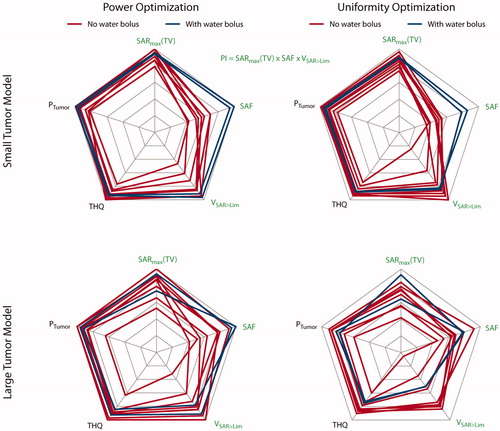
Figure 5. Top row: sagittal, coronal and axial section through the large tumor model. Left: description and front view of each design simulated together with the large tumor model; maximum intensity projection of the SAR_10g distribution after hyperthermia treatment planning for the power optimization (center) and the uniformity optimization (right).

Restivo MC, van den Berg CAT, van Lier ALHMW, et al. Local specific absorption rate in brain tumors at 7 tesla. Magn Reson Med. 2016;75(1):381–389.

 PubMed Web of Science ®Google Scholar

Gabriel C. Compilation of the dielectric properties of body tissues at RF and microwave frequencies. DTIC Document; 1996.

 Google Scholar

Athey TW, Stuchly MA, Stuchly SS. Measurement of radio frequency permittivity of biological tissues with an open-ended coaxial line: part I. IEEE Trans Microwave Theory Techn. 1982;30(1):82–86.

 Web of Science ®Google Scholar

Stuchly MA, Athey TW, Samaras GM, et al. Measurement of radio frequency permittivity of biological tissues with an open-ended coaxial line: part II—experimental results. IEEE Trans Microwave Theory Techn. 1982;30(1):87–92.

 Web of Science ®Google Scholar