Advanced patient-specific hyperthermia treatment planning

Figures & data

Figure 1. Workflow describing schematically all the methodological steps performed for advanced HTP. In HTP preparation, the patient anatomical model is obtained from CT segmentation. The vasculature, reconstructed from an MR scan and registered to the CT, is also included in this model. The dielectric properties are assigned to each tissue type based on the median DL-EPT values. The thermal properties are assigned from literature values, but an effective thermal conductivity accounting for convective heat transfer in the bladder is assigned. Next, treatment planning is performed, in which the electric field distribution is calculated and phase-amplitude settings for effective tumor heating are optimized. Finally, biological modeling predicts the radiosensitizing effect of hyperthermia in terms of an equivalent enhanced radiation dose.

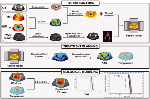
Table 1. Electrical and thermal properties of pelvic tissues at 70 MHz.

	Conductivity σ (Sm^–1)^a	Permittivity εr (rel. units)	Density ρ (kg m^–3)	Specific heat capacity ct (J kg^–1 K^–1)	Thermal conductivity kt (W m^–1 K^–1)	Perfusion Wb (kg m^–3 s^–1)
Air	0	1	1.29	10000^b	0.024	0
Bladder	1.22	50	1024	4178	5.6^c	0
Blood	0.83	84.1	1050	3617	0.52	–
Bone	0.12	16.4	1908	1313	0.32	0.12
Fat	0.04	13.4	911	2348	0.21	1.1
Muscle	0.91	70.8	1090	3421	0.49	3.6
Cervical tumor	1.02	70.8	1090	3421	0.49	1.8

Bold font indicates the parameters that were introduced in this study and differing from literature values (in normal font).

^a The values of σ obtained with DL-EPT at 128 MHz were decreased by 3% to determine the values at 70 MHz.

^b The value of c_t for air is ten times higher to permit larger time steps in thermal computations. This has a negligible effect on the steady state temperature.

^c The value of k_t for bladder was ten times higher than the literature value to account for convection phenomena in the bladder.

Table 2. Parameters and 95% confidence intervals (within brackets) used in the EQD_RT calculation expressed in Equation (5(5) $${\mathit{EQD}}_{RT}=D·\frac{\frac{\alpha \left(37\right)}{\beta \left(37\right)}·\hspace{0.17em}\text{exp}\hspace{0.17em}\left[\frac{T-37}{41-37}·ln\left(\frac{\alpha \left(41\right)}{\alpha \left(37\right)}\right)\right]+G·D·\hspace{0.17em}\text{exp}\hspace{0.17em}\left[\frac{T-37}{41-37}·ln\left(\frac{\beta \left(41\right)}{\beta \left(37\right)}\right)\right]}{\frac{\alpha \left(37\right)}{\beta \left(37\right)}+d_{\mathit{ref}}}+\frac{\frac{\alpha \left(37\right)}{\beta \left(37\right)}·\left[7.38·{10}^{13}·\left(T+273.15\right)·\hspace{0.17em}\text{exp}\hspace{0.17em}\left(\frac{\Delta S}{2}-\frac{\Delta H}{2·\left(T+273.15\right)}\right)\right]}{\alpha \left(37\right)·\left(\frac{\alpha \left(37\right)}{\beta \left(37\right)}+d_{\mathit{ref}}\right)}$$(5) ).

Parameter (measure unit)	Value
α(37) (Gy^–1)	0.386 (0.364 − 0.409)
α(37)/β(37) (Gy)	17.9 (14.6 − 22.5)
α(41)/α(37) (–)	1.73 (1.64 − 1.83)
β(41)/β(37) (–)	0.41 (0.28 − 0.59)
ΔS (cal/°C/mol)	392.08 (391.62 − 392.46)
ΔH (cal/mol)	147907.8 (NA)^a

These values were obtained from SiHa cervical cancer cell line experiments [62]. ^aΔH has no confidence interval since it is a fixed parameter.

Figure 2. DL-EPT. Transverse and coronal cross-section of MR magnitude image from AFI sequence, |B₁⁺| map, transceive phase (ϕ^±) map, conductivity map obtained with DL-EPT (σ_DL). |B₁⁺| and ϕ^± maps are given as input to the trained network, which infers σ_DL. The tumor contour is shown in red. The tumor was delineated by a radiation oncologist on an ADC map (part of the diagnostic MRI protocol) [85,86]. The tumor delineation was then rigidly transferred to the frame of reference of the AFI image.

Figure 3. Histograms of DL-based conductivity in pelvic tissues. Conductivity histograms are reported for each tissue along with the median value (black dashed line). Conductivity histograms were based on conductivity values within manually delineated tissue ROIs, depicted on the MR magnitude image (bladder: yellow; bone: blue; fat: magenta; muscle: green; tumor: red).

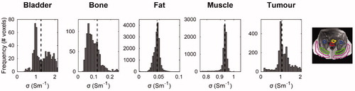
Figure 4. Vessel definition on MR and CT scans. Vessel delineations are shown on the transverse and coronal cross-sections of water image generated with the DIXON method (left) and on the HT-CT scan (right). These delineations were manually adjusted after MR to CT registration (not shown). At the bottom, a 3D rendering of the final vessel tree is shown.

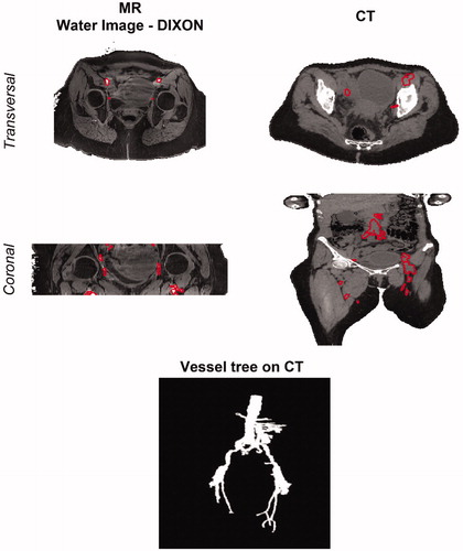
Figure 5. Patient model, SAR and Temperature maps. Transverse, sagittal and coronal cross-sections of the segmented model (first row), showing all the tissues included in the patient model, the SAR distribution (second row) and the temperature distribution (third row) in the patient. The GTV contour is indicated in black.

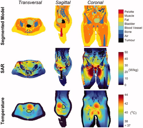
Figure 6. Equivalent dose distributions in radiotherapy and radiotherapy plus hyperthermia. Transverse, sagittal and coronal cross-sections of the radiotherapy (RT) dose distribution (first row), the temperature distribution obtained from hyperthermia treatment planning (second row), and the equivalent dose distribution derived from combining radiotherapy and hyperthermia (third row). The equivalent radiation dose was calculated within the GTV, which is denoted with blue contours. NB: The high-dose region adjacent to the GTV reflects an additional lymph node boost (with mean dose of 54.59 Gy).

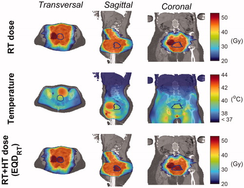
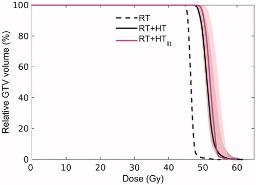
Figure 7. Dose Volume Histogram (DVH) reflecting the dose distribution in the GTV for radiotherapy alone (RT, dashed black line) and the combined radiotherapy and hyperthermia treatment as predicted with the advanced HTP workflow (RT + HT, solid black line). For comparison, the DVH predicted using a routine HTP workflow based on literature dielectric properties is also shown (RT + HT_lit, solid magenta line). The shaded area around the DVH for RT + HT and RT + HT_lit corresponds to confidence intervals resulting from uncertainty in LQ parameters.

van Leeuwen CM, Oei AL, ten Cate R, et al. Measurement and analysis of the impact of time-interval, temperature and radiation dose on tumour cell survival and its application in thermoradiotherapy plan evaluation. Int J Hyperthermia. 2018;34(1):30–38.

 PubMed Web of Science ®Google Scholar

de Boer P, Spijkerboer AM, Bleeker MCG, et al. Prospective validation of craniocaudal tumour size on MR imaging compared to histoPAthology in patients with uterine cervical cancer: the MPAC study. Clin Transl Radiat Oncol. 2019;18:9–15.

 PubMed Web of Science ®Google Scholar

Lim K, Small W, Portelance L, et al. Consensus guidelines for delineation of clinical target volume for intensity-modulated pelvic radiotherapy for the definitive treatment of cervix cancer. Int J Radiat Oncol Biol Phys. 2011;79(2):348–355.

 PubMed Web of Science ®Google Scholar