The impact of data selection and fitting on SAR estimation for magnetic nanoparticle heating

Figures & data

Figure 1. Schematic of adiabatic, and non-adiabatic heating curves during the heating (coil on) and cooling (coil off) phases of a heat experiment. Common fitting time-frames to calculate SAR_v include: Time-Rise, Box-Lucas, Steady State, and Decay.

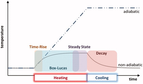
Figure 2. Effect of variation in SAR_v and RMSE using Box-Lucas and Time-Rise fitting as a function of SAR_v. Red circles indicate higher variation of SAR_v and RMSE caused by measurements performed in a sub-optimal heating range. The blue square indicates the range with a consistent SAR_v despite fitting method.

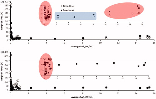
Figure 3. Evaluation and start time impact on SAR_v and RMSE. Plots A and B show the impact of evaluation time on SAR_v and RMSE when the start time is selected at 5s after heating. The SARv values are compared with the average SAR_v across all 12 fitting scenarios. A higher impact in both variation of SAR_v and RMSE is observed with Time-Rise fitting. Figure 3C evaluates the percentage difference in SAR between (1) SAR_v calculated excluding the first 5 s and (2) SAR_v calculated including t = 0-5 in the selected data range. Similarly, 3D evaluates the percentage difference in RMSE between these two cases. In this case, Box-Lucas fitting is observed to have larger variations in both SARv and RMSE than variations observed with Time-Rise fitting.

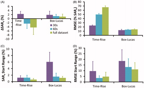
Figure 4. Repeatability of SARv measurement. Plot A shows the standard deviation of the replicate measurements as a function of evaluation time (using 5s start time) for SAR_v ≤ 0.1 W/mL. Plot B right shows the standard deviation of the replicate measurement as a function of evaluation time for SAR_v ≥ 0.1 W/mL. An increase in variation is observed at lower SAR_v. Furthermore, the R2 optimization results in more variable results than a statistically set evaluation time.

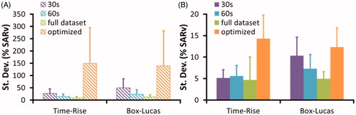
Table 1. Recommended parameters to report^a.

SARv (W/mL)	Recommendation
< 1	For high noise, Time-Rise use RMSE to guide selection of the evaluation time, and report criteria used to select the time interval for analysis of heating data
	For low noise -> Either Method
1–10	Both methods work, report selected method and use RMSE to guide selection of evaluation time and start time
> 10	Box-Lucas, use RMSE to guide start time; expect inaccuracy if dataset is shortened due to physical sample constraints (i.e. boiling).

^aSAR_v ranges given are specific to Bordelon et al. & Etheridge et al. and will vary based on heating losses in the experimental setup.

Table 2. Recommended parameters to report.

Sample	Experimental setup	Calculation parameters	Reported calculations
Volume (≥ 2 mL) Sample holder Matrix (tissue, cells, or solution) IONP concentration [15] Method of cFe determination [22,23]	Coil (geometry and # of turns) [8,14,28] Temperature probe (type & placement) [14,16,17] Insulation Sample placement in coil [8,27] Magnetic field frequency Magnetic field amplitude Uniform field VOI	Fitting method Start point selection Evaluation time Number of replicate measurements	SARv or SLP RMSE of fit Standard deviation of replicate measurements

Lahiri BB, Ranoo S, Philip J. Uncertainties in the estimation of specific absorption rate during radiofrequency alternating magnetic field induced non-adiabatic heating of ferrofluids. J Phys D: Appl Phys. 2017;50(45):455005.

 Web of Science ®Google Scholar

Hedayati M, Abubaker-Sharif B, Khattab M, et al. An optimised spectrophotometric assay for convenient and accurate quantitation of intracellular iron from iron oxide nanoparticles. Int J Hyperthermia. 2018;34(4):373–381.

 PubMed Web of Science ®Google Scholar

Ring HL, et al. Ferrozine assay for simple and cheap iron analysis of silica-coated iron oxide nanoparticles. ChemRxiv. 2018.

 Google Scholar

Zhang J, Ring HL, Hurley KR, et al. Quantification and biodistribution of iron oxide nanoparticles in the primary clearance organs of mice using T1 contrast for heating. Magn Reson Med. 2017;78(2):702–712.

 PubMed Web of Science ®Google Scholar

Wildeboer RR, Southern P, Pankhurst QA. On the reliable measurement of specific absorption rates and intrinsic loss parameters in magnetic hyperthermia materials. J Phys D: Appl Phys. 2014;47(49):495003.

 Web of Science ®Google Scholar

Wang SY, Huang S, Borca-Tasciuc DA. Potential sources of errors in measuring and evaluating the specific loss power of magnetic nanoparticles in an alternating magnetic field. IEEE Trans Magn. 2013;49(1):255–262.

 Web of Science ®Google Scholar

Makridis A, Curto S, van Rhoon GC, et al. A standardisation protocol for accurate evaluation of specific loss power in magnetic hyperthermia. J Phys D: Appl Phys. 2019;52(25):255001.

 Web of Science ®Google Scholar

Skumiel A, Hornowski T, Józefczak A, et al. Uses and limitation of different thermometers for measuring heating efficiency of magnetic fluids. Appl Therm Eng. 2016;100(Supplement C):1308–1318.

 Web of Science ®Google Scholar

Huang S, Wang S-Y, Gupta A, et al. On the measurement technique for specific absorption rate of nanoparticles in an alternating electromagnetic field. Meas Sci Technol. 2012;23(3):035701.

 Web of Science ®Google Scholar