Vein wall shrinkage induced by thermal coagulation with high-intensity-focused ultrasound: numerical modeling and in vivo experiments in sheep

Figures & data

Figure 1. Illustration of the HIFU transducer positioning on the site of interest.

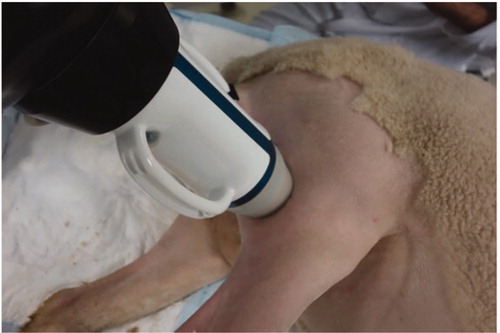
Figure 2. Illustration of the HIFU exposures (orange crosses) on a site and definition of the frame of reference with respect to the anatomy.

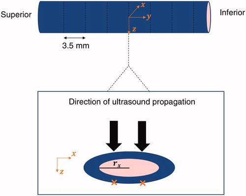
Figure 3. Flowchart of the methodology followed to model the vein wall shrinkage. The ultrasound propagation is first modeled using the k-wave library. From the acoustic simulations, the temperature evolution in tissues is dynamically estimated during the treatment. Based on the updated temperature field, the thermal damage to the vein is computed and the geometry of the vein is updated.

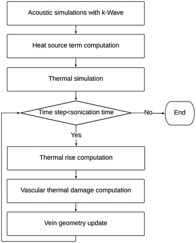
Table 1. Acoustic properties of tissues used for simulations.

	Cooling liquid	Superficial tissues	Muscles	Blood	Vein wall
Sound speed (m s^−1)	1495	1573 [21]	1580 [22]	1580	1580
Density (kg m^−3)	1000	995 [21]	1060	1060 [23], [24]	1060
Attenuation at 3 MHz (dB cm^−1)	0.02 [25]	2.48 [21]	2.25 [22]	0.5 [22]	4.35 [26]
Acoustic non-linearity parameter	5 [27]	7.8 [21]	7.8 [22]	7.8	7.8

Figure 4. Evolution of the vein contraction with Ω.

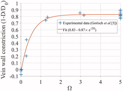
Figure 5. Illustration of thermal damage and vein wall constriction process. The vein wall is represented here by concentric rings of blue pixels, having each a unitary length. Based on the updated temperature field modeled by the Pennes bioheat equation, the thermal damage within each voxel is updated ${\mathrm{\Omega }}_{\mathrm{inter}}$ and the vein wall constriction ($\mathrm{\Lambda }$) is computed. The weighed curvilinear abscissa is then calculated and updated. Based on the special mean of the contracted pixel length, the new venous circumference is computed and the new geometry of the vein is updated. Finally, the thermal damage within each pixel of the updated vein wall is computed.

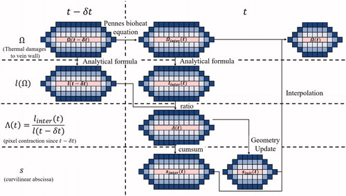
Figure 6. Post-treatment measurements of vein diameters.

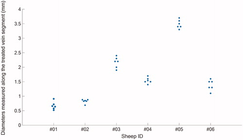
Table 2. Vein diameter reduction measurements.

Sheep ID	Blood flow visible during sonications?	Vein diameter before treatment^a, leg lowered (mm)	Vein diameter before treatment^a, leg elevated (mm)	Vein diameter post treatment, leg elevated (mm)	Diameter constriction (%)
#01	No	5.3 ± 0.1	2.3 ± 0.1	0.7	68
#02	No	5.2 ± 0.2	2.3 ± 0.2	0.8	64
#03	Yes	4.7 ± 0.3	3.7 ± 0.1	2.2	40
#04	No	3.8 ± 0.1	3.5 ± 0.1	1.5	58
#05	Yes	6.2 ± 0.2	5.2 ± 0.1	3.5	32
#06	No	3.5 ± 0.1	3.3 ± 0.3	1.4	58

^aAverage value reported.

Figure 7. Ultrasound images of a sheep vein before (a) and immediately after HIFU treatment (b) showing luminal shrinkage and blurred vascular contours.

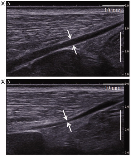
Figure 8. Simulated rms pressure field of the geometrical model in the $xz$ plane. Pressure is expressed in MPa. Yellow rectangles represent the limits of the subsequent layers.

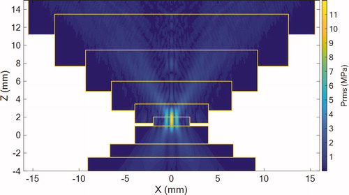
Figure 9. Shrinkage and thermal damage simulations for veins with an initial pretreatment diameter of 2.3 mm (top row), 3.5 mm (middle row) and 5.2 mm (bottom raw) after exposures of the vein. Left column: before treatment. Left column: after treatment. Note that the number of “yellow” pixels does not reflect the percentage of vein wall which is damaged since these pixels correspond to shrunken part of the vein wall. Typically, for the 5.2 mm vein, the coagulated pixels correspond to about 50 % of the initial vein wall.

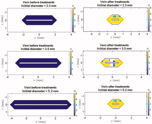
Figure 10. Comparison between the simulated (blue) and experimental (red) luminal shrinkage in one vein cross-section. The error bars refer to the experimental standard deviations ($\sigma$) and means are represented by the red circles.

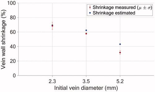
Table 3. Relative errors for the three diameters studied.

Semi-major axis length at the beginning of the treatment	Shrinkage estimated for the three diameters
	2.3 mm	3.5 mm	5.3 mm
Semi-major axis length at the beginning of the treatment unchanged (rx)	69.4%	62.4%	43.2%
Semi-major axis length at the beginning of the treatment with an error of +11%	69.4%	64.5%	47.8%
Relative errors (${\mathit{\delta }}_{1.11{\mathit{r}}_{\mathit{x}}}$)	0.06%	−3.3%	−10.6%

Grisey A, Heidmann M, Letort V, et al. Influence of skin and subcutaneous tissue on *High-intensity focused ultrasound beam: experimental quantification and numerical modeling. Ultrasound Med Biol. 2016;42(10):2457–2465.

 PubMed Web of Science ®Google Scholar

Duck FA. Physical properties of tissues: a comprehensive reference book. London: Academic Press; 1990.

 Google Scholar

Xu F, Lu TJ, Seffen KA, et al. Mathematical modeling of skin bioheat transfer. Appl Mech Rev. 2009;62(5):050801.

 Web of Science ®Google Scholar

Solovchuk MA, Thiriet M, Sheu TWH. Computational study of acoustic streaming and heating during acoustic hemostasis. Appl Therm Eng. 2017;124:1112–1122.

 Web of Science ®Google Scholar

Wang S, Frenkel V, Zderic V. Preliminary optimization of non-destructive high intensity focused ultrasound exposures for hyperthermia applications. Proceedings of the 31st Annual International Conference of the IEEE Engineering in Medicine and Biology Society, 2009. p. 3055–3059.

 Google Scholar

Kim M, Kim J-Y, Noh S-C, et al. Thermal characteristics of non-biological vessel phantoms for treatment of varicose veins using high-intensity focused ultrasound. PLoS One. 2017;12(4):e0174922.

 PubMed Web of Science ®Google Scholar

Gianmarco P. Numerical methods for nonlinear wave propagation in ultrasound. Durham: Duke University; 2007.

 Google Scholar