Challenges and recommendations for magnetic hyperthermia characterization measurements

Figures & data

Table 1. Field frequency, intensity and sample volume parameters chosen as the best match for the different capabilities of the measurement laboratories.

Frequency	Field intensity	Sample volume
300 kHz	15 kAm^−1 (Peak) − 10.6 kAm^−1 (RMS)	1 ml

Table 2. Properties of the liquid suspensions distributed for measurement: c_FeOx = iron oxide concentration; σ_s = saturation magnetization per unit mass of iron oxide, measured at 300 K; M_s = saturation magnetization per unit volume of iron oxide, measured at 300 K; d_core = average magnetic core diameter; d_Hydro = intensity (z) average hydrodynamic diameter; PDI = polydispersity index; the latter two parameters determined from second order cumulant fitting of the DLS correlogram.

Sample ID	cFeOx [mgFeOx/mL]	σs [Am^2/kgFeOx]	Ms [kA/m]	dcore [nm]	dHydro [nm]	PDI
Sample 1	40.6	69.3	356	7.0	170	0.21
Sample 2	3.9	94.4	485	8.3	90	0.24

Figure 1. As-reported SLP values for Samples 1 and 2 plotted against CSM-recalculated values. The CSM analysis takes account of the inherent environmental losses in non-adiabatic calorimetry systems and is confined to the ‘linear loss region’ of the T(t) heating curves. The dotted line is a best linear fit to the data; it has a slope of ca. 1.15, indicating a tendency for the as-reported values to be higher than the recalculated ones.

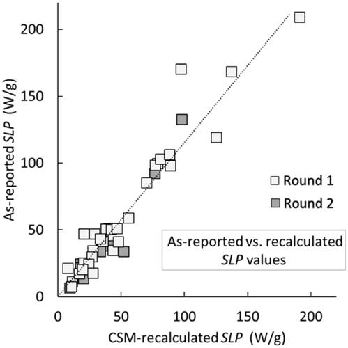
Figure 2. SLP values for Samples 1 and 2 plotted as a function of H_o² f, for which at least a monotonic trend is expected, according to Equations (1)(1) $$\mathit{SLP}=P/m_{\text{MNP}},$$(1) and (3)(3) $$P={\mu }_{0}f\oint M\left(t\right)\mathrm{ }\mathrm{d}{H}_{}\left(t\right),$$(3) . The scatter evident in the data points is an indication of interlaboratory measurement variability. Dotted lines are guides to the eye only.

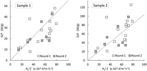
Figure 3. Mandel h statistics (relative to the mean) for Round 1 measurements, using the CSM-recalculated ILP values. Laboratory 1 is an outlier, with h values that exceed the ± 0.5% significance level, h_crit = 2.51.

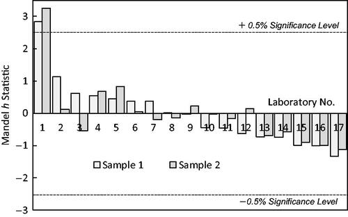
Figure 4. Youden plots of CSM-recalculated ILP values for both samples and for both rounds of measurement. The vertical and horizontal dashed lines mark the mean values for each sample, ILP_1-mean and ILP_2-mean. The diagonal line has slope ILP_2-mean/ILP_1-mean $\simeq$ 2.25.

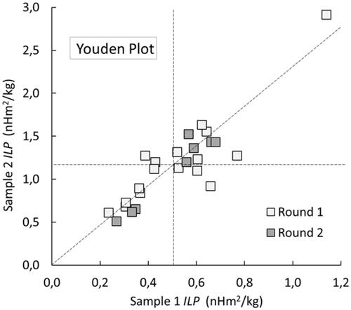
Figure 5. Interlaboratory rank correlation of the CSM-recalculated ILP values for both samples and both rounds of measurement. Each data point represents the ranking of a pair of measurements (ILP_1, ILP₂) recorded in a single laboratory in a single round. The dotted line corresponds to the best linear fit to the data; its slope is equal to the Spearman correlation coefficient for the data, ρ = 0.81.

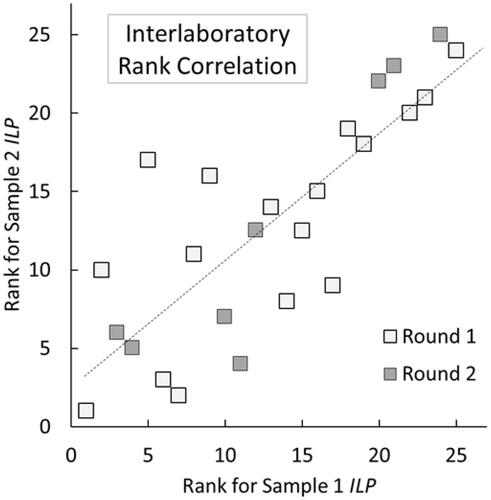
Table 3. Means and standard deviations of the as-reported and CSM-recalculated ILP values for Samples 1 and 2, for both rounds of the study.

Intrinsic Loss Power, ILP [nHm^2 kg^−1]	As-reported ILP values				CSM-recalculated ILP values
	Round 1		Round 2		Round 1		Round 2
	Sample 1	Sample 2	Sample 1	Sample 2	Sample 1	Sample 2	Sample 1	Sample 2
Mean	0.52	1.13	0.49	1.07	0.49	1.09	0.50	1.09
Std. dev.	0.14	0.42	0.14	0.45	0.15	0.30	0.16	0.42

Data from the outlier, Laboratory 1, identified in Figure 3, was excluded from these calculations. Round 1 data was therefore from N = 16 laboratories; Round 2 from N = 8 laboratories.

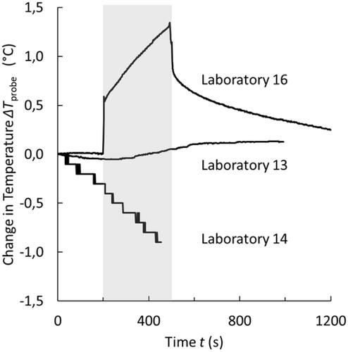
Figure 6. Illustration of the range of environmental heat transfer conditions under which different laboratory calorimeters operate, as measured using a centrally supplied pure water sample and the same measurement protocols as would be applied to a magnetic hyperthermia sample. The gray box highlights the period during which the magnetic field was applied. The middle curve is representative of the response recorded in most laboratories; the other two curves illustrate extreme responses.

Data availability statement

The data that support the findings of this study are publicly available for download. The files are uploaded in the Zenodo repository under the title “Radiomag Interlaboratory Comparison of Magnetic Hyperthermia Characterisation Measurements: Data” DOI: https://zenodo.org/record/4281154#.YEiMBk6g82w.