Figures & data
Figure 1. (a) Schematic of the computational model considered in the study computational model consists of three concentric cylindrical domains with the innermost domain being the gel phantom, the second layer being the water jacket and the outermost being the magnetic coil. (b) Sample mesh plot of the computational domains. (c) Three locations along the radius where temperatures were compared.
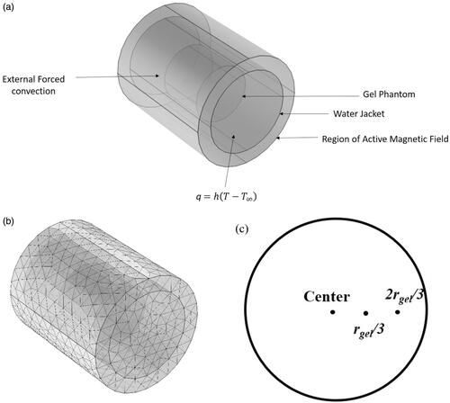
Table 1. Mean parameter values and their uncertainties considered in the simulations.
Figure 2. Experimental setup for the gel phantom experiments. Agar gel phantoms were inserted in the center of a 20-cm horizontal modified Maxwell coil inside a water jacket with temperature controlled at 20 °C. Temperatures were measured at the center of the gel, rgel/3, and 2rgel/3 distance along the radius of the gel, where r is the gel radius.
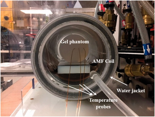
Figure 3. Workflow for building 3 D models of rabbit liver from CT scan images: CT scan images of rabbit liver were first imported into Slicer3D and the liver was extracted by manual segmentation. The file was then imported into MeshLab for meshing and smoothing of sharp edges to allow for import into finite element software for simulations. File was then imported into COMSOL via mesh import option and converted into geometry. The geometry is then remeshed in COMSOL and multi-physics is added for simulations.
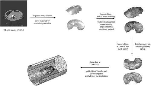
Figure 4. Schematic of the computational model used for simulations. (a) Isometric projection of the geometry showing the liver, tumor and rabbit tissue/torso. Thermal and magnetic field boundary conditions are shown. (b) Sample mesh for the computational model shown in (a).
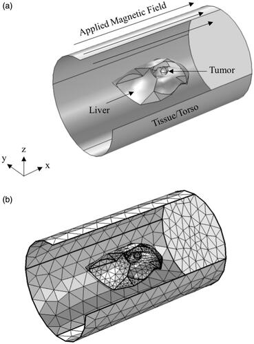
Table 2. Thermal properties of tissues considered in the present study.
Table 3. Electrical properties of tissue used in the simulations.
Figure 5. (a) Isothermal contours showing the temperature distributions achieved inside the phantom after 15 min of exposure to an alternating magnetic of 13.97 kA/m at a fixed frequency of 160 kHz, (b) verification of computational model with analytical solution. Comparison of computed temperatures with the coupled electromagnetic and heat transfer model with temperatures calculated using the analytical expression for power absorption at center of gel shows excellent agreement.
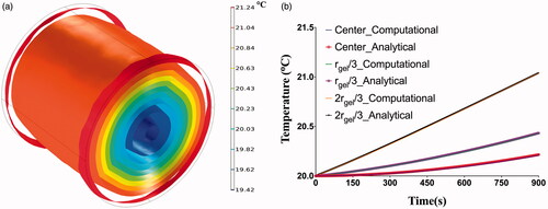
Figure 6. Overall uncertainty in temperatures as a function of time measured at the center, rgel/3, and 2rgel/3, due to uncertainty in individual parameters identified in . The variation in overall uncertainty of temperature with time was plotted for each probe location. Computed temperatures are most sensitive to the uncertainties in applied field (H), frequency (f), probe placement (Probe), specific heat capacity (Cp), electrical conductivity (σ) and gel density (ρ). Note r_1 and r_2 represent rgel/3, and 2rgel/3, respectively.
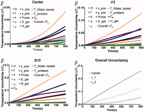
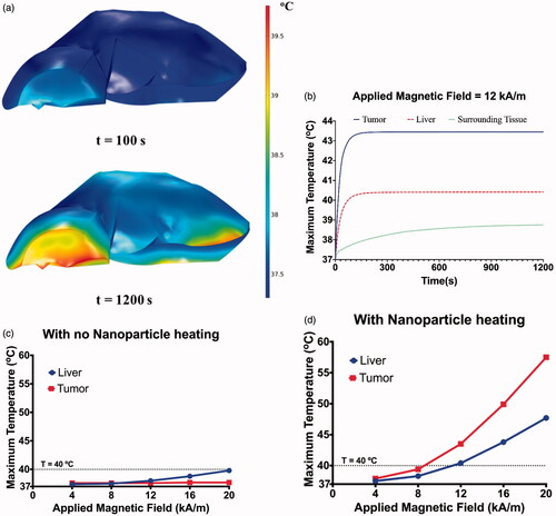
Figure 7. (a) Temperature distribution in the liver after 20 min of exposure to an AMF amplitude of 20 kA/m (peak) at a fixed frequency of 150 kHz. Elevated temperatures can be observed at the edges of the liver with temperature of ∼40 °C at the end of 20 min of exposure. (b) Maximum temperatures achieved in the tumor, liver and surrounding superficial tissue during 20 min of AMF exposure at 12 kA/m and 50 kHz. Maximum temperatures achieved in the liver and tumor after 20 min of exposure to an AMF amplitude of 4 to 20 kA/m (peak) at a fixed frequency of 150 kHz with (c) no nanoparticle heating and (d) with nanoparticle heating.