
Figures & data
Figure 1. Schematic for the methodology used to estimate patient treatability. Inputs include the anatomical patient MR images (representative slices shown here), the three exposure points (magenta), the tumor segment (red), and the covered (i.e., device reachable) tumor volume (yellow overlaid on the tumor segment). The transducer (blue) is positioned and angled such that the geometric focus was placed at reachable exposure points. In step 1, simulation grids are extracted from the larger MR image datasets. In step 2, each grid voxel is assigned acoustic and thermal properties using thresholds. A density image is displayed, with white denoting the densest material (bone) and black denoting the least dense material (oil) in the image. In step 3, an acoustic simulation is performed in order to estimate the acoustic pressure field within the complex distribution of tissues. The pressure field, overlaid on the density map and segmented tumor, shows regions of high (yellow) and low (blue) pressure. In step 4, thermal simulation identifies where tissue ablation should result from acoustic energy absorption and heat transfer. The thermal dose delivered to tissue is calculated. In Step 5, the patient treatability is estimated by examining the positions and volumes of ablated tissues (cyan) for the three exposure points in order to identify the maximum treatable depth, and hence, the treatable tumor volume (output).
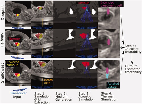
Table 1. Patient details.
Figure 2. The simulation grid (left) extracted from the original patient MR image is segmented into different tissues and materials (right). Physical properties (i.e., density, sound-speed, attenuation coefficient, thermal conductivity, specific heat capacity) were assigned to each voxel based on their tissue/material. For exposure points in which the transducer (blue, left) is situated outside the original patient MR image field-of-view, as in the case in this example (patient P3, halfway exposure point), all voxels outside the original patient MR image field-of-view were assigned the properties of the Sonalleve® oil (black region, right).
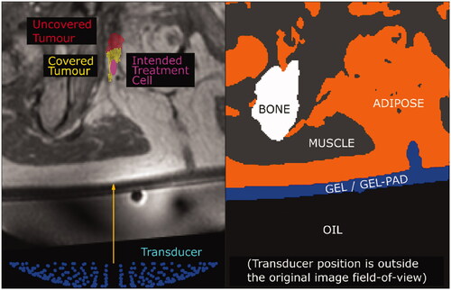
Table 2. Material properties for acoustic and thermal simulation.
Figure 3. Transducer used as the source for the acoustic simulations. The 256 6 mm-diameter elements are arranged in a bowl with an outer diameter of 138 mm, 140 mm geometric focal length and an inner hole of 44 mm in diameter.
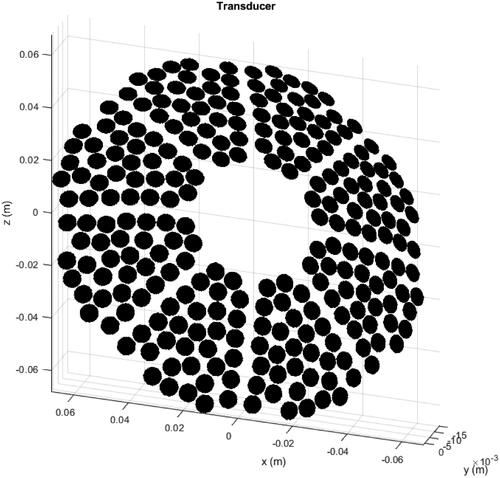
Table 3. Clinical treatment details for each patient.
Figure 4. Schematic diagram illustrating the calculation of the maximum treatable depth. Ablated tissue volume was linearly interpolated as a function of position (depth) between the greater and lesser ablated tissues in order to find the ‘cell-equivalent’ point, where the ablated tissue volume was interpolated to be 84 mm3. The maximum treatable depth was defined to be half a treatment cell length (5 mm for a 4 mm diameter cell) deeper than this point.
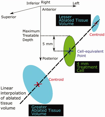
Figure 5. Representative cross-sections of simulated acoustic pressure fields (colour bar, only pressures >10% of focal peak pressure are shown) overlaid on the density map (grayscale, lighter means denser, that is, bone is white and oil is black) used for different patients and exposure points. The intended treatment cell (magenta, 4 mm wide, 10 mm long, centered at the geometric focus) is also shown relative to the tumor (red). Each cross-section is the slice in which the peak focal pressure lies.
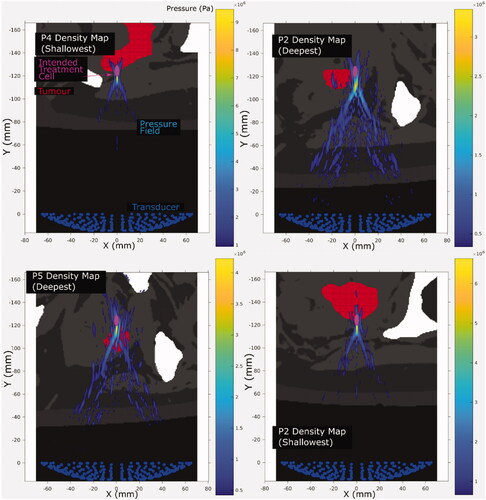
Figure 6. Cross sections of the ablated tissue (cyan), resulting from simulated sonication of the deepest, shallowest and halfway reachable treatment cells (magenta, 4 mm wide and 10 mm long centered at the geometric focus), overlaid on patient anatomy (grayscale in-phase MR image). The image slices are those with the largest ablated cross-sectional area. The ablated tissue volumes’ distances from the geometric focus, in all three dimensions, are quantified in .
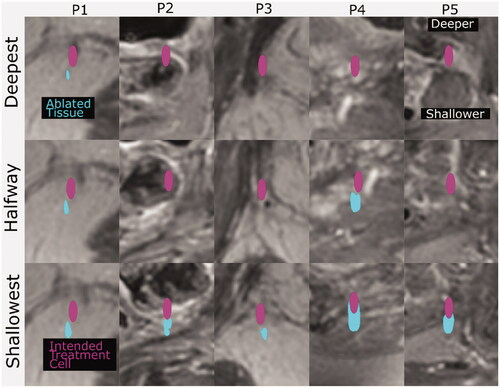
Table 4. Results of acoustic and thermal simulations.
Figure 7. Focal peak pressure (top), ablated tissue volume (middle) and Y-offset (bottom) dependence on beam path length in tissue. The dotted lines are linear regressions, with the squared correlation coefficients (R2) shown for each regression.
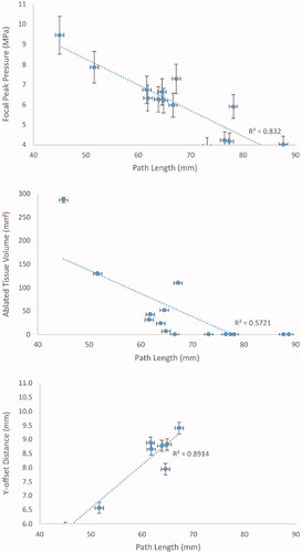
Figure 8. (P1–P5) Cross sections of the predicted treatable volume (cyan), predicted tumor coverage (yellow) and the remaining uncovered and untreatable tumor volume (red) overlaid on patient anatomy (greyscale in-phase MR image). The image slices are those at the position where the interpolated ablated tissue volumes are equal to the expected treatment cell volume (84 mm3). The transducer (138 mm aperture width) is shown for scale.
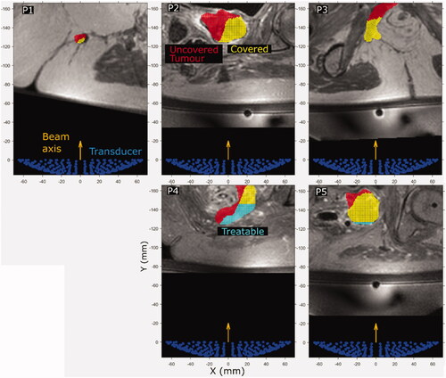
Table 5. Predicted tumor treatable volume compared with clinically treated volume and predicted tumor coverage volume.
Data availability statement
The data that support the findings of this study are not available due to limitations in the ethical review.