Figures & data
Figure 1. Geometric models utilized in this study. (a) A tissue-mimicking leg phantom was constructed to mimic a sheep tibia with metal plates affixed to the cortical bone with screws. The leg and plates were embedded in a tissue-mimicking gel phantom and housed in a cylindrical container. Fiber-optic temperature sensors were attached to different faces of the plates as well as in the bone phantom and gel material. (b) A sheep model with the same plates was used to test AMF exposures in vivo, with a corresponding simulation model of the leg incorporating bone, muscle, fascial layers, and skin. Both geometries had corresponding simulation models as shown.
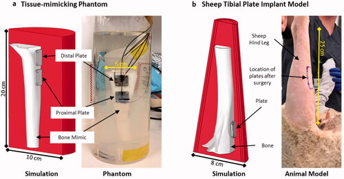
Figure 2. (a) A driving system was developed to power the AMF coils. The system was mobile and had an articulating arm to hold the AMF coil at a desired orientation around the sheep. (b) The solenoid coil is shown with the corresponding capacitors used to form a parallel tank circuit. Both the capacitors and coil were cooled with the water circuit. (c) An impedance matching circuit comprised of a series inductor and parallel capacitor were placed in between the amplifier and the tank circuit to enable efficient power transfer to the coil.
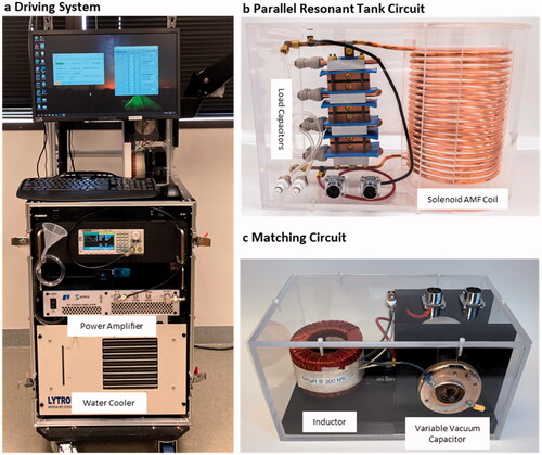
Figure 3. Validation of numerical simulations with phantom data. (a) Volumetric temperature distribution around the implant plate at different timepoints with the dotted red lines showing the cutout location from the volume. (b) Overlaying comparison between simulated and recorded phantom heating curves for a multiple pulse AMF sequence with 14 s exposure with 300 s delay. The points A, B, and C to the time points in a. (c) Correlation between ΔT achieved in simulations and phantom heating for different exposure times on both implant plates, gel, and bone mimic (left to right respectively).
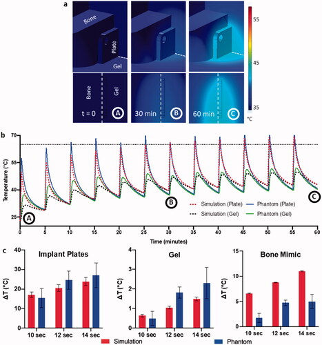
Figure 4. Experimental model for temperature measurement studies in sheep model. (a) Graphical depiction in front and side view of sheep leg for temperature sensor placement. (b) Pictures from surgery with placement of implant plate and sensors going through the hoof and a view after suturing. Temperature readings from all 5 sensors during (c) single 10 s AMF exposure and (d) temperature readings from plate sensors for multiple pulse 10 s AMF exposure with a 325 s delay.
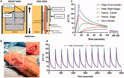
Figure 5. Validation of numerical simulations with temperature data from sheep model. Comparison of temperature evolution between simulation and sheep model for AMF heating, texp=10 s, on (a) implant surface, and (b) in the surrounding tissue. Summarizing the correlation between simulated temperature prediction and experimental data at multiple timepoints encompassing heating and cooldown periods for the above AMF heating for c plate sensors and d fascia and skin sensors.
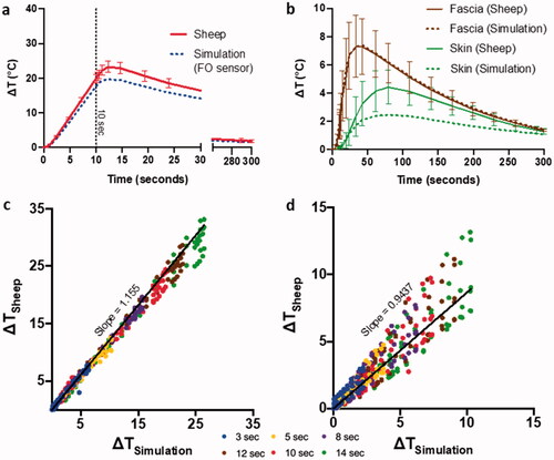
Figure 6. Simulation of sheep leg and temperature sensitivity of implant plates to movement within coil with AMF heating. Exposure duration = 8 s and Tmax=65 °C. (a) The 3D simulation model showing the solenoid coil capable of producing uniform field in Z-axis, along with limb, bone, implants, axis directions and rotation about center of mass (white dot). (b) Simulated surface temperature distribution at various timepoints for AMF heating. (c) Bar graph with median and inter-quartile range for temperature distribution on the top implant plate at different positions within the coil for AMF heating.
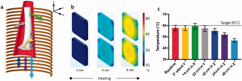
Figure 7. Construction and characterization of the AMF system. (a) Circuit diagram with connections between each component of the AMF system. Function generator provides an input voltage to the amplifier. Amplified current (I1) passes through the 50 Ω matching circuit. Current is magnified inside the tank circuit (I2) resulting in AMF. (b) Peak magnetic field strength at coil center versus peak coil current and power delivered to the AMF system needed to generate each current (blue dots). (c) Simulation of tank circuit and the magnetic field it generates. Peak values (mT) are color-coded along magnetic field lines. Simulated and measured variation in magnetic field with change in position along coil axis and distance from center of coil.
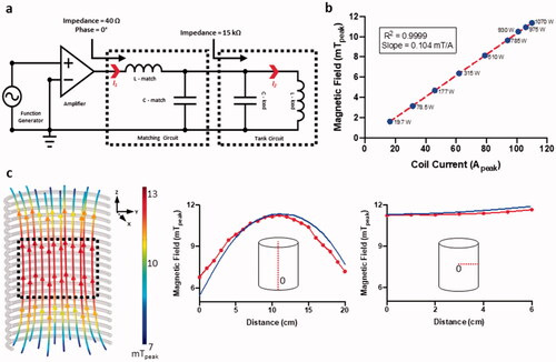
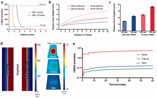
Table 1. To account for different in temperature measured with fiberoptic sensors to the actual temperature of the plate, a correction factor is devised.
Figure 8. Simulation of thermal dose accumulation on and around the implant with AMF exposure. (a) Spatial distribution of CEM43 thermal dose in muscle tissue near the implant after 1 and 12 pulses of for AMF heating, Tmax, implant=65 °C (Ti=32 °C). Thermal dose in the implant while targeting 65 °C and reducing pulse delay from 300 to 150 s (b) progressing during the 12 pulses, and (c) at the end of 12th pulse. (d) 3D thermal dose distribution on the surface and cross-section of bone, fascia, and skin (log color range) after 12 pulses of AMF heating, exposure duration = 10 s and Tmax, implant t=65 °C. (e) Predicted evolution of thermal dose on bone, fascia and skin during corresponding to center of implant plate for the whole AMF exposure. Ti: initial temperature.