Figures & data
Figure 1. System setup for ex vivo as well as in vivo ablations with MRIT temperature monitoring.
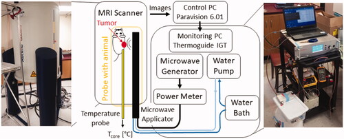
Figure 2. Custom made directional MRI-compatible applicator. (A) geometry of radiating tip. (B) Photo of applicator together with close-up view of the distal radiating tip of the applicator and proximal part with electrical connection and water inflow and outflow lines.
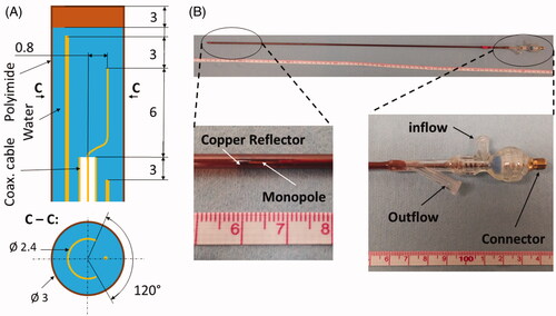
Figure 3. Holding template (A) for phantom or ex vivo tissue in MRI scanner. Axial slices of phantom (B) and chicken breast (C) samples loaded in template along with marked positions of applicator and fiber optic sensors.
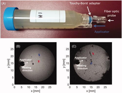
Figure 4. Example (A–C) anatomic MR images of subcutaneously implanted HAC15 tumors (red contour) and the microwave ablation applicator (white arrow). The boundaries of all six treated tumors (D) in a central axial plane through the tumor.
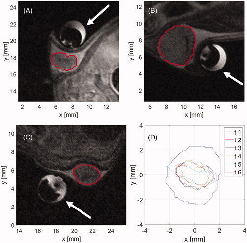
Figure 5. T2-turboRare anatomical image with highlighted positions of axial slices for real-time temperature monitoring.
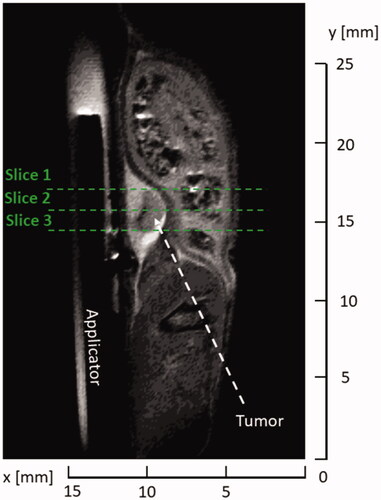
Figure 6. Comparison of simulated ablation zone at 30 W (A,C) and 50 W (B,D) input power (as measured at the power meter) with target tumor boundaries in a central axial plane. While (A,B) illustrate sample temperature distributions and tumor boundaries, (C,D) provide the Dice Similarity Coefficient (DSC) between the simulated extent of the ablation zone and the corresponding tumor boundary, for each of the six cases. White space in (A,B) denotes the applicator. Solid lines in (A,B) denote the tumor boundary and dashed lines represent the CEM43 = 240 min isodose line.
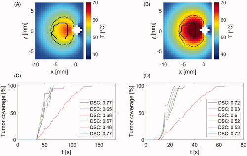
Figure 7. Comparison of temperature profiles during heating in agar phantom (B) and chicken breast (D) along with magnitude images (A,C) with position of applicator, heating direction and positions of fiber optic probes (circle marks) and regions of interest (square marks) for temperature evaluation. Magnitude images also show temperature maps, which were achieved at 240 s after the start of heating. The color of temperature difference curves shown in (B,D) correspond to the color of location markers in magnitude images (A,C).
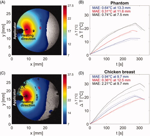
Figure 8. (A) Magnitude image showing the tumor and surrounding anatomy and control points used for temperature monitoring and terminating procedure when temperature reaches threshold of 55 °C. (B) Temperatures estimated at control points shown in subfigure (A). Color of each line corresponds to color of control point in subfigure (A).
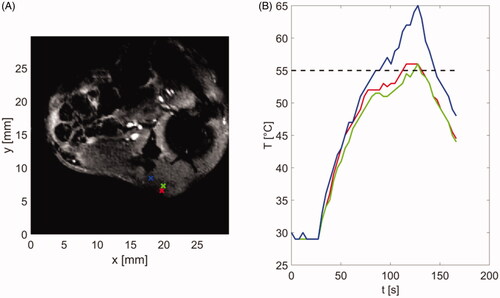
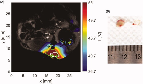
Table 1. Achieved coverage of tumor by thermal dose of at least 240 CEM43 and maximum estimated temperature in tumor for 5 out of 6 mice.
Figure 9. (A) Sample temperature map shown over the magnitude image at the end of ablation. White contour stands for segmented tumor and green contour for area with thermal dose greater than 240 CEM43. (B) Extracted tumor with applied TTC staining (white tissue) and surrounding vessels (red tissue).