Figures & data
Figure 1. From patient imaging to patient model (patient 10): (a) an axial slice of the patient MRI; (b) the segmentations on the same slice of bone, muscle, skin, tumor, and fibroglandular-fat mixture; (c) the same segmentation on the same slice, with the automated division of the fibroglandular-fat mixture into two distinct tissue entities; (d) the two-component GMM that lead to the selected cutoff value in the fibroglandular and fat mixture.
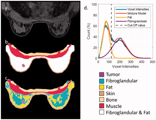
Figure 2. Top 3D view of all 22 generated breast cancer models. All models are on the same scale.
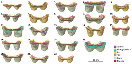
Figure 3. Graphic representation of the tumor position classifications. Five distinct tumor positions are assumed: upper outer; upper inner; lower outer; lower inner; and central tumor position.
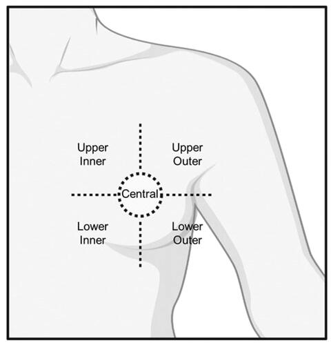
Table 1. Summary of patient and tumor characteristics.
Figure 4. Treatment planning setup and results in a single patient (Patient 10). (a) The water bolus and dipole antennas positions (red dots) distributed along two rings around the breast tissue; (b) tissue discretization in an axial slice passing through the center of the tumor; (c) normalized 1 g averaged SAR distribution on the same slice after THQ optimization; (d) steady-state temperature distribution on the same slice.
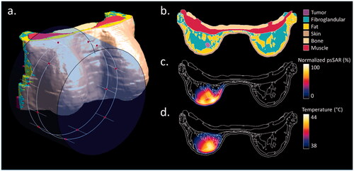
Table 2. Assigned physical, electrical, and thermal tissue properties.
Figure 5. Boxplots of the hyperthermia treatment planning parameters on all patients; (a) the THQ; (b) the TC25, TC50, and TC75; (c) the T10, T50, and T90.
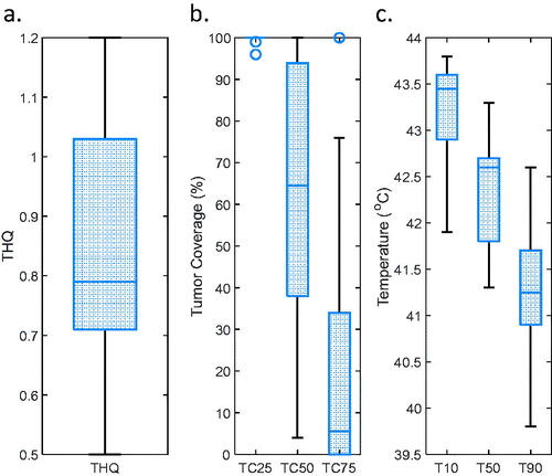
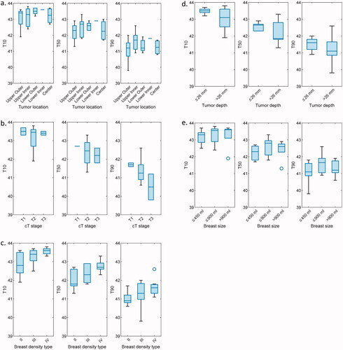
Figure 6. Evaluation of the tumor temperature volume metrics (T10, T50, T90) for different anatomical and tumor characteristics: (a) between different tumor location groups; (b) between different tumor stage groups; (c) between different breast density types; (d) between deep and superficial tumor locations; (e) between different breast sizes (≤450 ml; >450 ml & ≤900 ml; >900 ml).