Validating a simulation model for laser-induced thermotherapy using MR thermometry

Figures & data

Figure 1. MR imaging of the experimental setup in axial (a) and coronary (b) orientation. MR images show the liver in the center (1), the agarose gel phantoms in the periphery (2), the laser applicator (3), the plastic tube (4) passing through the liver (partial representation of the plastic tube in a), and bloodless vessels (5). A schematic in axial orientation with the position of the MR slice is shown in (c). The artificial vessel is positioned at right angles to the applicator and the MR imaging plane.

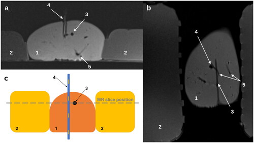
Figure 2. Sketch of the computational domain Ω and the boundary decomposition: radiating surface of the applicator ${\Gamma }_{\text{rad}},$ cooled surface of the applicator ${\Gamma }_{\text{cool}},$ surface of the artificial blood vessel ${\Gamma }_{\text{vessel}},$ and ambient surface of the liver ${\Gamma }_{\text{amb}}.$

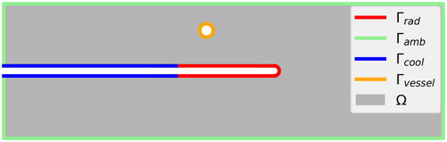
Table 1. Experimental setup for the test cases.

Label	Case 1	Case 2	Case 3	Case 4
Laser Power ${\widehat{q}}_{\text{app}}$ [W]	20	20	20	20
Time laser on $t_{\text{on}}$ [s]	60	60	60	60
Temperature [${}^{°}$C]
-initial $T_{\text{init}}$	16.0	17.5	17.5	18.0
-coolant $T_{\text{cool}}$	20.0	20.0	20.0	20.0
-vessel $T_{\text{vessel}}$	20.5	20.5	20.5	20.5
-ambient $T_{\text{amb}}$	21.8	20.8	20.5	20.8
Distance [mm]
-applicator/tube	6	9	8	8

Table 2. Modeling parameters for simulating ex-vivo porcine liver tissue with an artificial blood vessel.

Parameter	Value	Source
Optical (native)
Absorption coefficient μan [m^–1]	50	[29]
Scattering coefficient μsn [m^–1]	8000	[29]
Anisotropy factor gn	0.97	[29]
Absorption factor βqn	0.14	[5]
Optical (coagulated)
Absorption coefficient μac [m^–1]	60	[29]
Scattering coefficient μsc [m^–1]	30000	[29]
Anisotropy factor gc	0.95	[29]
Absorption factor βqc	0.35	Fitted
Thermal
Thermal conductivity κ [W m^–1 K^–1]	0.518	[30]
Heat capacity Cp [J kg^–1 K^–1]	3640	[30]
Tissue density ρ [kg m^–3]	1137	[30]
Heat transfer coefficient ${\alpha }_{\text{cool}}$ [W m^–2 K^–1]	250	Fitted
Heat transfer coefficient ${\alpha }_{\text{vessel}}$ [J mol^–1 K^–1]	3500	Fitted
Damage
Damage rate constant A [s^–1]	3.1 ${\times }^{98}$	[31]
Damage activation energy Ea [J mol^–1 K^–1]	$6.3\times {10}^5$	[31]
Universal gas constant R [J mol^–1 K^–1]	8.31	[31]

Table 3. Positions of the applicator and the artificial vessel.

Case Label	Case 1	Case 2	Case 3	Case 4
Applicator
–tip ${\mathbf{p}}_{\text{app}}$ [mm]	(105.6, 120.0, 2.5)	(114.5, 155, 0)	(98.1, 145.3, 1)	(111.3, 131.3, 0)
–direction ${\mathbf{d}}_{\text{app}}$	(0.089, 0.995, 0.042)	(0.033, 0.999, 0)	(-0.115, 0.993, 0.003)	(-0.080, 0.997, 0)
Vessel
–point ${\mathbf{p}}_{\text{vessel}}$ [mm]	(109.3, 86.8, 0)	(122.6, 124.9, 0)	(109.5, 132.7, 0)	(105.3, 114.8, 0)
–direction ${\mathbf{d}}_{\text{vessel}}$	(0, 0, 1)	(0, 0, 1)	(0, 0, 1)	(0, 0, 1)

Figure 3. Case 1: Comparison between measured $T_{\exp }$ and simulated temperature $T_{\text{sim}}.$ The standard deviation σ is computed within the dashed box, disregarding the hatched area where the measurement is unreliable due to coagulation.

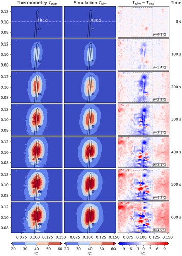
Figure 4. Case 2: Comparison between measured $T_{\exp }$ and simulated temperature $T_{\text{sim}}.$ The standard deviation σ is computed within the dashed box, disregarding the hatched area where the measurement is unreliable due to coagulation. Note: For this case artifacts in the MR thermometry data likely result in faulty temperature measurements.

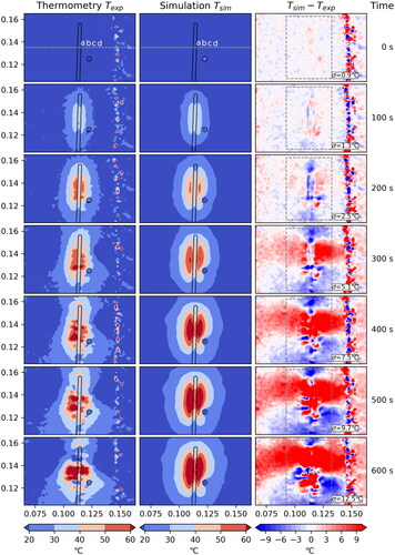
Figure 5. Case 3: Comparison between measured $T_{\exp }$ and simulated temperature $T_{\text{sim}}.$ The standard deviation σ is computed within the dashed box, disregarding the hatched area where the measurement is unreliable due to coagulation.

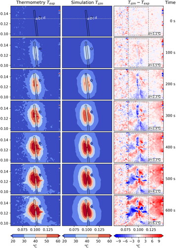
Figure 6. Case 4: Comparison between measured $T_{\exp }$ and simulated temperature $T_{\text{sim}}.$ The standard deviation σ is computed within the dashed box, disregarding the hatched area where the measurement is unreliable due to coagulation. Note: For this case artifacts in the MR thermometry data likely result in faulty temperature measurements.

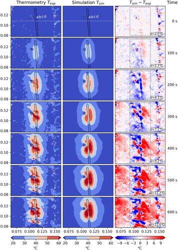
Figure 7. One-dimensional plot over the line shown in Figures 3–6 to compare measured and simulated temperatures at different time steps during the experiments.

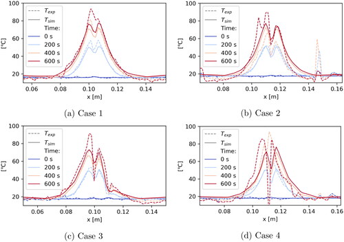
Figure 8. Plot over time at the points a, b, c and d (Figures 3–6) to compare measured and simulated temperatures.

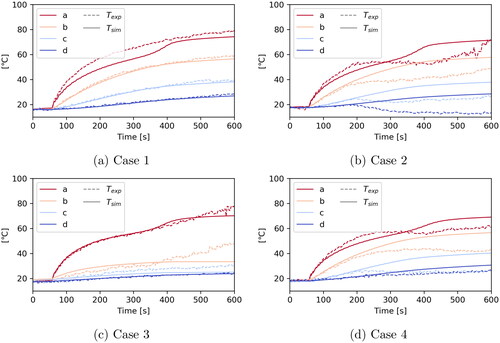
Table 4. Mean temperatures ${\overline{T}}_{\exp }$ and ${\overline{T}}_{\text{sim}}$ as well as standard deviation σ in regions of interest (ROI) with radius 5 mm around the vessel (Ω_V) and contralateral to the vessel (Ω_C), i.e. around the position of the vessel mirrored by the applicator.

		ROI	0 s	100 s	200 s	300 s	400 s	500 s	600 s
Case1	${\overline{T}}_{\exp }$	ΩV	16.1	21.9	27.4	30.1	30.7	30.3	30.3
		ΩC	16.0	24.8	36.4	41.9	46.3	46.7	48.6
	${\overline{T}}_{\text{sim}}$	ΩV	17.4	23.0	26.1	27.6	28.6	29.2	29.5
		ΩC	16.0	24.4	35.1	41.6	46.0	48.8	50.5
	σ	ΩV	1.7	1.6	3.7	5.4	6.8	8.3	9.4
		ΩC	0.6	1.0	1.2	3.7	7.2	6.5	5.1
Case2	${\overline{T}}_{\exp }$	ΩV	17.7	22.8	29.0	31.8	33.1	34.1	34.3
		ΩC	17.8	23.7	34.4	40.5	46.5	49.6	43.6
	${\overline{T}}_{\text{sim}}$	ΩV	18.4	23.1	26.9	28.7	29.8	30.4	30.7
		ΩC	17.5	23.5	33.7	40.7	45.5	48.1	49.7
	σ	ΩV	1.3	2.1	4.6	4.3	4.1	5.5	7.4
		ΩC	0.7	1.1	1.6	3.2	5.2	6.6	16.4
Case3	${\overline{T}}_{\exp }$	ΩV	17.9	21.6	26.6	29.2	29.9	31.4	32.9
		ΩC	17.5	22.7	33.0	43.2	49.1	53.7	56.9
	${\overline{T}}_{\text{sim}}$	ΩV	18.4	22.9	27.1	29.1	30.4	31.0	31.2
		ΩC	17.5	23.5	34.3	42.0	47.0	49.5	51.1
	σ	ΩV	1.1	1.5	3.0	4.0	5.0	5.5	7.6
		ΩC	1.0	1.2	1.1	1.6	1.9	2.2	3.0
Case4	${\overline{T}}_{\exp }$	ΩV	19.5	26.4	35.8	37.3	36.9	37.2	37.8
		ΩC	18.2	26.0	39.0	43.3	44.1	44.2	45.2
	${\overline{T}}_{\text{sim}}$	ΩV	18.8	25.2	29.6	31.5	33.2	34.3	34.8
		ΩC	18.0	27.3	40.8	49.2	54.9	57.9	59.4
	σ	ΩV	8.5	6.6	11.5	23.9	24.2	31.2	37.1
		ΩC	0.7	1.5	2.9	3.8	3.7	4.7	6.7

Roggan A, Dorschel K, Minet O, et al. The optical properties of biological tissue in the near infrared wavelength range. In Laser-induced interstitial therapy. Bellingham (WA): SPIE Press; 1995. p. 10–44.

 Google Scholar

Hübner F, Leithäuser C, Bazrafshan B, et al. Validation of a mathematical model for laser-induced thermotherapy in liver tissue. Lasers Med Sci. 2017;32(6):1399–1409.

 PubMed Web of Science ®Google Scholar

Giering K, Minet O, Lamprecht I, et al. Review of thermal properties of biological tissues. In Laser-induced interstitial therapy. Bellingham (WA): SPIE Press; 1995. p. 45–65.

 Google Scholar

Schwarzmaier H-J, Yaroslavsky IV, Yaroslavsky AN, et al. Treatment planning for mri-guided laser-induced interstitial thermotherapy of brain tumors–the role of blood perfusion. J Magn Reson Imaging. 1998;8(1):121–127.

 PubMed Web of Science ®Google Scholar