HYPER: pre-clinical device for spatially-confined magnetic particle hyperthermia

Figures & data

Figure 1. Opposing magnets create a strong magnetic field gradient containing a FFR that provides the basis for spatially-confined heating with the HYPER prototype. The volume of the FFR depends on gradient strength, where a stronger gradient creates a smaller FFR. When and AMF is applied, the nanoparticles within the FFR (region A) are free to generate thermal energy due to hysteresis losses; however, outside the FFR (region B), the magnetic moments of the nanoparticles are fixed and contribute little to heating.

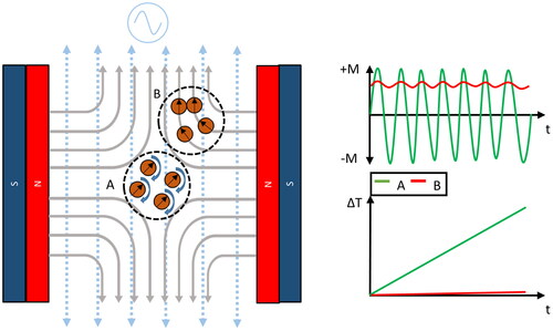
Figure 2. Three-dimensional computer-aided design (CAD) models of the magnet and RF assembly of the HYPER system. (a) Isometric view of the magnet assembly; (b) top view (normal to y-axis) of the HYPER without exterior paneling. This view shows the permanent magnets along the x-axis, the RF coil assembly, the tuning circuitry, and the sample platform. (c) Front view (normal to z-axis) of the HYPER without exterior paneling. From this angle, the y-axis stage is visible.

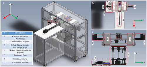
Figure 3. Heating sequence programming using the graphic user interface (GUI). (a) the GUI enables the user to execute a spatially-confined heating plan entered as command lines. The user first selects the ROIs in 3D space on the sample using the bi-planar camera views: AP and LAT, and the program generates a preset plan in the configuration editor; (b) Flow chart outlining the processes that occur during a measurement with the HYPER.

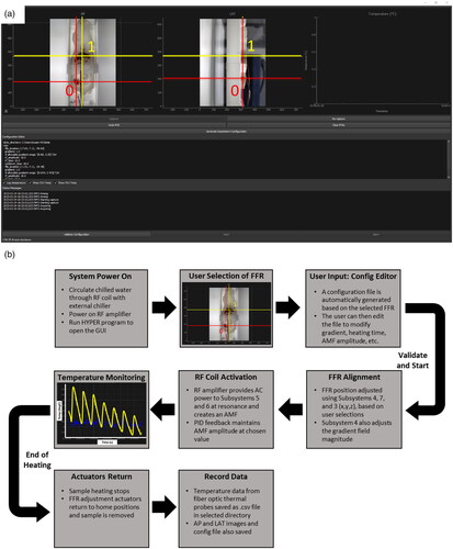
Figure 4. Assembled hyper prototype. (a) In addition to the magnet and AMF assembly, the system includes a rack containing control systems, an RF amplifier, a water chiller, and animal heater. The chiller circulates water through the RF coil, with temperature that can be varied between 20 °C and 40 °C. The animal heater circulates water through the sample stage during in vivo experiments to maintain the core body temperature of the mouse models. (b) Diagram of the sample stage orientation within the HYPER, denoted by the dashed box.

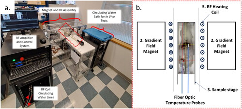
Figure 5. Thermal PSF at five gradient strengths along all three axes. A nanoparticle sample was heated at varying positions along the x, y, and z-axis relative to the FFR, located at the isocenter. Thermal PSF at varying gradients along (a) x-axis; (b) y-axis; (c) z-axis. (d) Upon fitting the thermal PSFs to the derivative of the Langevin function, we calculated the FWHM in each dimension for the tested particles.

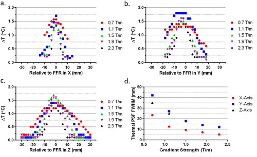
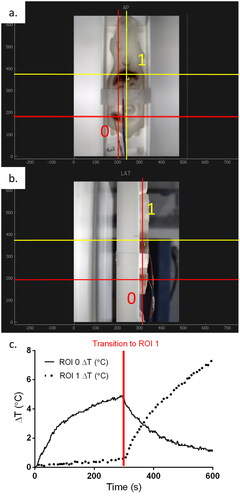
Figure 6. Verification of spatially confined heating with mouse phantom. Regions of interest ROI 0 (red) and ROI 1 (yellow) were selected in the HYPER GUI from both the top (a) and side (b) views. (c) Sequential heating of ROI 0 and ROI 1 is demonstrated. Despite both ROIs existing within the RF coil, the gradient field limits observed heating to the selected ROI.

Data availability statement

The data that support the findings of this study are available from the corresponding author, H.C., upon reasonable request.