Bayesian rank-based hypothesis testing for the rank sum test, the signed rank test, and Spearman's ρ

Figures & data

Figure 1. The graphical model underlying the Bayesian rank sum test. The latent, continuous scores are denoted by $Z_i^x$ and $Z_i^y$, and their manifest rank values are denoted by $x_i$ and $y_j$. The latent scores are assumed to follow a normal distribution governed by the parameter δ. This parameter is assigned a Cauchy prior distribution, which for computational convenience is reparameterized to a normal distribution with variance g (which is then assigned an inverse gamma distribution).

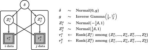
Figure 2. The relationship between the latent normal Bayes factor and the observed rank-based test statistic is illustrated for logistic data. Because U is dependent on n, the rank biserial correlation coefficient is plotted on the x-axis instead of U. The relationship is clearly defined, and maximum evidence in favor of ${\mathcal{H}}_0$ is attained when ${\rho }_{rb}=0$. The further ${\rho }_{rb}$ deviates from 0, the stronger the evidence in favor of ${\mathcal{H}}_1$ becomes. The lines depict smoothing splines fitted to the observed Bayes factors.

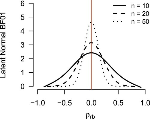
Figure 3. For all combinations of difference in location parameters Δ, and n, the relationship between the latent normal Bayes factor and the parametric Bayes factor is shown for logistic data. The black lines indicate the point of equivalence. The two Bayes factors are generally in agreement, as suggested by the ARE results in [58].

Figure 4. Do students who flunk a math course report drinking more alcohol? Results for the Bayesian rank sum test as applied to the data set from [9]. The dashed line indicates the Cauchy prior with scale $\frac{1}{\sqrt{2}}$. The solid line indicates the posterior distribution. The two grey dots indicate the prior and posterior ordinate at the point under test, in this case $\delta =0$. The ratio of the ordinates gives the Bayes factor.

Table 1. The scores, difference scores, ranks of the absolute difference scores, and the sign indicator function Q for the hypothetical scenario where $X=(5,8,4)$ are the initial scores on a math exam and $Y=(6,7,7)$ are the scores on the exam after a tutoring session.

i	$(y_i-x_i)$	$d_i$	$\mathrm{r}\mathrm{a}\mathrm{n}\mathrm{k}(\mid d_i\mid )$	$Q\left(d_i\right)$
1	6−5	1	1.5	1
2	7−8	$-1$	1.5	$-1$
3	7−4	3	3	1

Figure 5. The graphical model underlying the Bayesian signed rank test. The latent, continuous difference scores are denoted by $Z_i^d$, and their manifest signed rank values are denoted by $d_i$. The latent scores are assumed to follow a normal distribution governed by parameter δ. This parameter is assigned a Cauchy prior distribution, which for computational convenience is reparameterized to a normal distribution with variance g (which is then assigned an inverse gamma distribution).

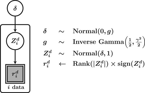
Figure 6. The relationship between the latent normal Bayes factor and the observed rank-based test statistic is illustrated for logistic data. Because W is dependent on n, the matched-pairs rank-biserial correlation coefficient is plotted on the x-axis instead of W. The relationship is clearly defined, and maximum evidence in favor of ${\mathcal{H}}_0$ is attained when ${\rho }_{mrb}=0$. The further ${\rho }_{mrb}$ deviates from 0, the stronger the evidence in favor of ${\mathcal{H}}_1$ becomes. The lines are smoothing splines fitted to the observed Bayes factors.

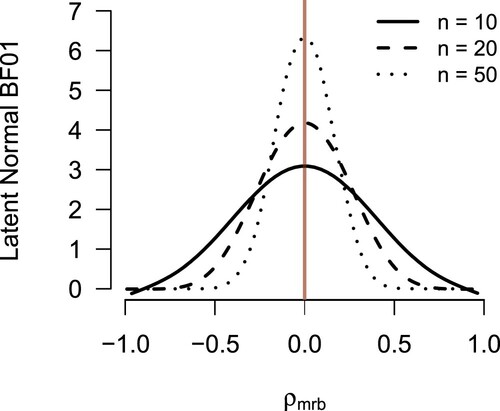
Figure 7. For all combinations of difference in location parameters Δ, and n, the relationship between the latent normal Bayes factor and the parametric Bayes factor is shown for logistic data. The black lines indicate the point of equivalence. The two Bayes factors are generally in agreement, with the latent normal Bayes factor accumulating evidence in favor of the true model faster.

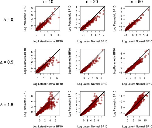
Figure 8. Does progabide reduce the frequency of epileptic seizures? Results for the Bayesian signed rank test as applied to the data set presented in [57]. The dashed line indicates the Cauchy prior with scale $\frac{1}{\sqrt{2}}$. The solid line indicates the posterior distribution. The two grey dots indicate the prior and posterior ordinate at the point under test, in this case $\delta =0$. The ratio of the ordinates gives the Bayes factor.

Figure 9. The graphical model underlying the Bayesian test for Spearman's ${\rho }_s$. The latent, continuous scores are denoted by $Z_i^x$ and $Z_i^y$, and their manifest rank values are denoted by $r_i^x$ and $r_j^y$. The latent scores are assumed to follow a normal distribution governed by parameter ρ (which is assigned a uniform prior distribution).

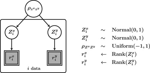
Figure 10. The relationship between the latent normal Bayes factor and the observed rank-based test statistic is illustrated for data generated with the Clayton copula. The relationship is clearly defined, and maximum evidence in favor of ${\mathcal{H}}_0$ is attained when Spearman's ${\rho }_s=0$. The further Spearman's ${\rho }_s$ deviates from 0, the stronger the evidence in favor of ${\mathcal{H}}_1$ becomes. The lines are smoothing splines fitted to the observed Bayes factors.

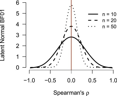
Figure 11. For all combinations of Spearman's ${\rho }_s$ and n, the relationship between the latent normal Bayes factor and the parametric Bayes factor is shown for data generated with the Clayton copula. The black lines indicate the point of equivalence. The two Bayes factors are generally in agreement.

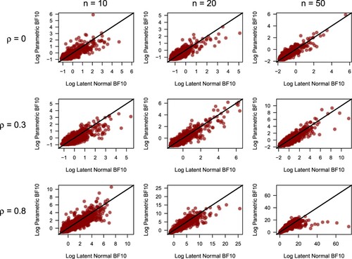
Figure 12. Is performance on a math exam associated with the quality of family relations? Results for the Bayesian version of Spearman's ${\rho }_s$ as applied to the data set from [9]. The dashed line indicates the uniform prior distribution, and the solid line indicates the posterior distribution. The two grey dots indicate the prior and posterior ordinate at the point under test, in this case $\rho =0$. The ratio of the ordinates gives the Bayes factor.

A. van der Vaart, Asymptotic Statistics, Cambridge Series in Statistical and Probabilistic Mathematics, Cambridge University Press, Cambridge, 2000.

 Google Scholar

P. Cortez and A.M.G. Silva, Using data mining to predict secondary school student performance, in Proceedings of 5th Annual Future Business Technology Conference, A. Brito and J. Teixeira, eds., EUROSIS, Porto, 2008, pp. 5–12.

 Google Scholar

P.F. Thall and S.C. Vail, Some covariance models for longitudinal count data with overdispersion, Biometrics 46 (1990), pp. 657–671. doi: https://doi.org/10.2307/2532086

 PubMed Web of Science ®Google Scholar