Bayes factor testing of equality and order constraints on measures of association in social research

Figures & data

Table 1. Examples of possible tests that can be executed using the proposed methodology.

	Example hypothesis test
Precise testing	$H_0:\rho =0$ versus $H_1:\rho \ne 0$
One-sided testing	$H_0:\rho \le 0$ versus $H_1:\rho >0$
Multiple hypothesis testing	$H_0:\rho =0$ versus $H_1:\rho <0$ versus $H_2:\rho >0$
Interval testing	$H_0:\left|\rho \right|\le .1$ versus $H_1:\left|\rho \right|>.1$
Equality-constrained testing	$H_1:{\rho }_{12}={\rho }_{13}={\rho }_{14}$ versus $H_2:`\mathrm{n}\mathrm{o}\mathrm{t}{H}_1$
Order-constrained testing	$H_1:{\rho }_{12}<{\rho }_{13}<{\rho }_{14}$ versus $H_2:{\rho }_{12}>{\rho }_{13}>{\rho }_{14}$ versus $H_3:`\mathrm{n}\mathrm{e}\mathrm{i}\mathrm{t}\mathrm{h}\mathrm{e}\mathrm{r}{H}_1,nor{H}_2^{\prime }$
Hypotheses with equality and order constraints	$H_1:{\rho }_{12}<{\rho }_{13}={\rho }_{14}$ versus $H_2:`\mathrm{n}\mathrm{o}\mathrm{t}{H}_1$

Table 2. Types of measures of association depending on the measurement scale of the variables.

	Scale of $Y_2$
	Dichotomous	Polychotomous-	Continuous-
Scale $Y_1$		Ordinal categories	Interval
Dichotomous	Tetrachoric	Polychoric	Biserial
Polychotomous-		Polychoric	Polyserial
Ordinal categories
Continuous-			Product-
Interval			Moment

Figure 1. Graphical model describing partial associations between life and domain satisfaction variables.

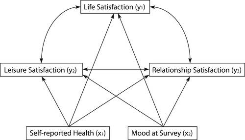
Table 3. Rough guidelines for interpreting Bayes factors [57].

$B_{12}$	Evidence
$<1/150$	Very strong evidence for $H_2$
1/150 to 1/20	Strong evidence for $H_2$
1/20 to 1/3	Positive evidence for $H_2$
1/3 to 1	Weak evidence for $H_2$
1	No preference
1 to 3	Weak evidence for $H_1$
3 to 20	Positive evidence for $H_1$
20 to 150	Strong evidence for $H_1$
$>150$	Very strong evidence for $H_1$

Figure 2. (a) Graphical representation of the subspace of $({\rho }_{21},{\rho }_{31},{\rho }_{32})$ for which the 3-dimensional correlation matrix is positive definite (taken from [59] with permission). The thick diagonal line from $(-\frac{1}{2},-\frac{1}{2},-\frac{1}{2})$ to $(1,1,1)$ represents the correlations that satisfy ${\rho }_{21}={\rho }_{31}={\rho }_{32}$ and result in a positive diagonal correlation matrix. (b) Uniform prior ${\pi }_1^U$ for the common correlation ρ under $H_1:{\rho }_{21}={\rho }_{31}={\rho }_{32}$ in the allowed region ${\mathcal{C}}_1=\{\rho |\rho \in (-\frac{1}{2},1\left)\right\}$. (c) Uniform prior ${\pi }_2^U$ for the free parameters under $H_2:{\rho }_{31}=0$ in the allowed region ${\mathcal{C}}_2=\left\{\right({\rho }_{21},{\rho }_{32})|{\rho }_{21}^2+{\rho }_{32}^2<1\}$. (d) Uniform prior for the free correlations under $H_3:{\rho }_{31}=0,{\rho }_{21}>{\rho }_{32}$ in the allowed region ${\mathcal{C}}_3=\left\{\right({\rho }_{21},{\rho }_{32})|{\rho }_{21}^2+{\rho }_{32}^2<1,{\rho }_{21}>{\rho }_{32}\}$.

Figure 3. Left panel. The implied $beta(\frac{1}{2},\frac{1}{2})$ prior in the interval $(-1,1)$ (dotted line) in the test proposed by Wetzels and Wagenmakers' [68], and the uniform prior in $(-1,1)$ as proposed here. Right panel. Implied prior for the common correlation ρ under $H_0:{\rho }_{12}={\rho }_{13}={\rho }_{23}$ when testing against $H_1:{\rho }_{12}\ne {\rho }_{13}\ne {\rho }_{23}$ using a marginally uniform encompassing prior (dotted line), and a uniform prior for ρ on $(-\frac{1}{2},1)$ (solid line) as proposed here.

Figure 4. Posterior probabilities of $H_1:{\rho }_{21}={\rho }_{31}={\rho }_{32}$ (solid line), $H_1:{\rho }_{21}>{\rho }_{31}>{\rho }_{32}$ (dotted line), and $H_2:$ not $H_1,H_2$ (dashed line) for different effects ρ and different sample sizes n.

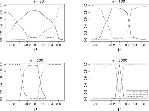
Table 4. Posterior probabilities for the competing hypotheses from Examples 1 and 2.

Application 1: Life, leisure,and relationship satisfaction
Hypothesis test 1	Posterior probabilities
$H_{1a}$: ${\rho }_{g1y2y1}>{\rho }_{g1y3y1}>{\rho }_{g1y3y2}$	0.0020
$H_{1b}$:${\rho }_{g1y3y1}>{\rho }_{g1y2y1}>{\rho }_{g1y3y2}$	0.0085
$H_{1c}$:${\rho }_{g1y3y1}={\rho }_{g1y2y1}={\rho }_{g1y3y2}$	0.9879
$H_{1d}$: neither $H_{1a}$, $H_{1b}$, nor $H_{1c}$	0.0016
Hypothesis test 2
$H_{2a}$: ${\rho }_{g2y2y1}>{\rho }_{g2y3y1}>{\rho }_{g2y3y2}$	0.0001
$H_{2b}$: ${\rho }_{g2y3y1}>{\rho }_{g2y2y1}>{\rho }_{g2y3y2}$	0.2955
$H_{2c}$: ${\rho }_{g2y3y1}={\rho }_{g2y2y1}={\rho }_{g2y3y2}$	0.2104
$H_{2d}$: neither $H_{2a}$, $H_{2b}$, nor $H_{2c}$	0.4940
Hypothesis test 3
$H_{3a}$: ${\rho }_{g1y2y1}>{\rho }_{g2y2y1}$	0.1588
$H_{3b}$: ${\rho }_{g1y2y1}={\rho }_{g2y2y1}$	0.8278
$H_{3c}$: ${\rho }_{g1y2y1}<{\rho }_{g2y2y1}$	0.0135
Hypothesis test 4
$H_{4a}$: ${\rho }_{g1y3y1}>{\rho }_{g2y3y1}$	0.0809
$H_{4b}$: ${\rho }_{g1y3y1}={\rho }_{g2y3y1}$	0.9017
$H_{4c}$: ${\rho }_{g1y3y1}<{\rho }_{g2y3y1}$	0.0174
Application 2: Support for justice principles
Hypothesis test 5
$H_{5a}$: ${\rho }_{g1y2y1}>{\rho }_{g2y2y1}>{\rho }_{g3y2y1}>{\rho }_{g4y2y1}$	0.0044
$H_{5b}$: ${\rho }_{g1y2y1}={\rho }_{g2y2y1}={\rho }_{g3y2y1}={\rho }_{g4y2y1}$	0.0000
$H_{5c}$: ${\rho }_{g1y2y1}={\rho }_{g2y2y1}>{\rho }_{g3y2y1}={\rho }_{g4y2y1}$	0.9899
$H_{5d}$: neither $H_{5a}$, $H_{5b}$, nor $H_{5c}$	0.0057

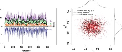
Figure A1. Left panel: Trace plot of latent $z_{31}$ observed in category 1 of the 3th (ordinal) outcome variable (blue line), $z_{32}$ observed in category 2 (orange line), $z_{33}$ observed in category 3 (green line), and $z_{34}$ observed in category 4 (purple line), as well as the corresponding threshold parameters ${\gamma }_{31}$, ${\gamma }_{32}$, and ${\gamma }_{34}$ for the 3th outcome variable. Right panel: Scatter plot of posterior draws of $({\eta }_{21},{\eta }_{31})$ (red dots) with additional contour plot and univariate density plots (solid lines) and normal approximations (dashed lines).

A.E. Raftery, Bayesian model selection in social research, Sociol. Methodol. 25 (1995), pp. 111–163.

 Web of Science ®Google Scholar

P.J. Rousseeuw and G. Molenberghs, The shape of correlation matrices, Am. Stat. 48 (1994), pp. 276–279.

 Web of Science ®Google Scholar

R. Wetzels and E.J. Wagenmakers, A default Bayesian hypothesis test for correlations and partial correlations, Psychon. Bull. Rev. 19 (2012), pp. 1057–1064.

 PubMed Web of Science ®Google Scholar