Figures & data
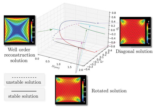
Figure 1. (a) A schematic of off-lattice HGO and GB models. The potential between two particles is described using their orientations ( and
) and relative position
. The width of each particle is set to
. (b) A schematic of lattice-based LL model. The orientation of particle i is given by
and the lattice spacing is set to
.
Figure 2. Typical configuration for HGO off-lattice model. After averaging over passes, the solutions are not stationary and the top and bottom rows show two example configurations. Plots on the left show a single particle configuration, while plots on the right show the spatially and temporally averaged s and director fields over the
passes. Parameters are
,
,
and
.
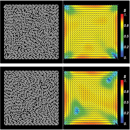
Figure 3. Typical configuration for HGO off-lattice model for a larger number, , of simulated molecules. The plot on the left shows a single particle configuration, while the plot on the right shows the spatially and temporally averaged s and director fields over the
passes. Other parameters are as in .
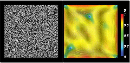
Figure 4. (a) Stationary configuration for HGO off-lattice model. Stationary s and director fields are obtained by averaging over an increased number of passes . Parameters are
,
,
and
. (b) Stationary configuration for the GB off-lattice model. Parameters are
,
,
,
,
,
,
,
and
.
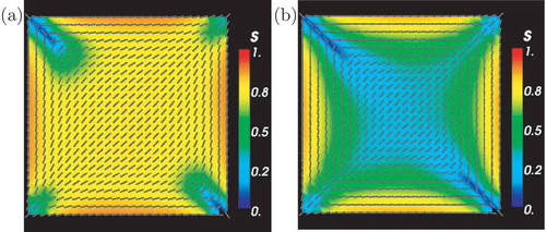
Figure 5. Typical configuration for GB off-lattice model. After averaging over passes, the solutions are not stationary and the top and bottom rows show two example configurations. Plots on the left show a single particle configuration, while plots on the right show the spatially and temporally averaged s and director fields over the
passes. Parameters are
,
,
,
,
,
,
and
.
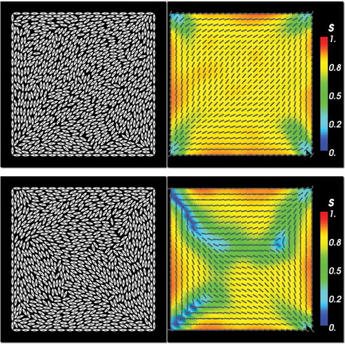
Figure 6. Sequence of averaged configurations showing switching between diagonal solutions in the GB off-lattice model. The plots show a sequence of three different averages, each using passes, over a total of
passes of the MCMC algorithm. Parameters are
,
,
,
,
,
,
and
.
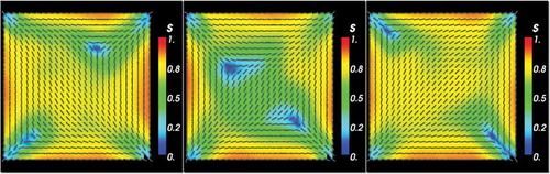
Figure 7. In each column, temperature parameter sweep for the lattice-based LL model. In each row, the MCMC simulations were run with either a D1-solution (left column) or a R1-solution (right column) of the continuum LdG model used as the initial condition. Each row corresponds with a different value for the (dimensionless and re-scaled) temperature T. Parameters are ,
and
.
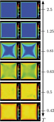
Table 1. Dirichlet boundary conditions resulting in optimal solutions D1–D2 and R1–R4.
Figure 8. Bifurcation solutions for the LdG model for a D1-solution (left column) and for a R1-solution (right column). The values for D for each column are
0.90, 1.20 μm. The tick marks on the D-axis show the approximate locations of the solution bifurcations, for example, the first bifurcation from the single stable WORS solution to the stable diagonal and unstable WORS solutions occurs at
.
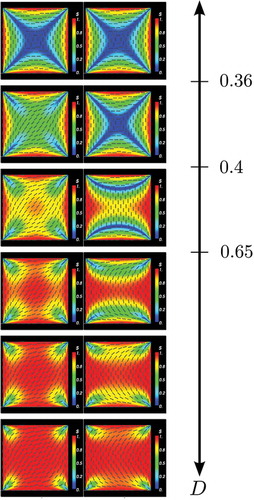
Figure 9. (Colour online) Total LdG energy for the R1 and D1 solutions plotted against domain size D. The blue/red lines correspond to the diagonal/rotated solutions presented in (left/right column). Solid lines indicate a stable solution branch, while dashed lines indicate an unstable solution branch.
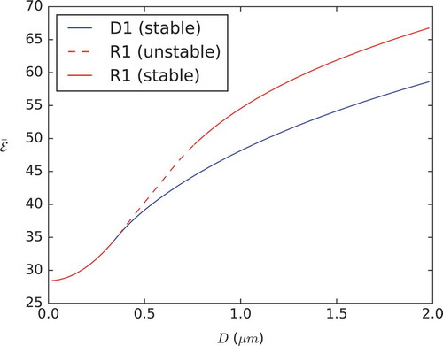
Table 2. The largest eigenvalue of the Jacobian of the RHS of equation Equations (4) and (5) is given here for each panel of , where the panel numbers are ordered from left to right and top to bottom.
Figure 10. (Colour online) Bifurcation diagram for the LdG model, plotting averaged quantities and
versus domain side D in order to show all the solution branches. (Top) Plot of
and
versus D. (Bottom) Orthogonal 2D projections of the full 3D plot. Solid red/blue lines: stable D1/D2 solutions. Solid black/purple/green/cyan lines: stable R1/R2/R3/R4 solutions. Dashed lines: unstable solutions leading to rotated branches. Solid dark cyan line (for
): stable WORS solution.
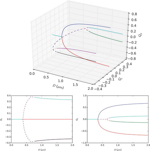
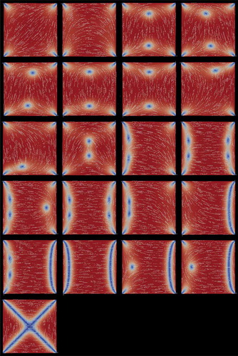
Figure 11. (Colour online) The deflation technique finds 81 equilibria for the LdG model at μm. Once rotational symmetries are discarded, 21 equilibria remain, which are depicted above ordered from left to right and top to bottom by the largest eigenvalue
of the Jacobian of the RHS of Equations (4) and (5) (values of
are given in ). The first two equilibria are the diagonal and rotated solutions, with negative eigenvalues (i.e. stable), the remainder have positive eigenvalues (i.e. unstable). The equilibria are shown coloured by the order parameter s (blue at
, increasing to red at
) and transparent white lines indicate the director direction n.