Elucidating the fine details of cholesteric liquid crystal shell reflection patterns

Figures & data

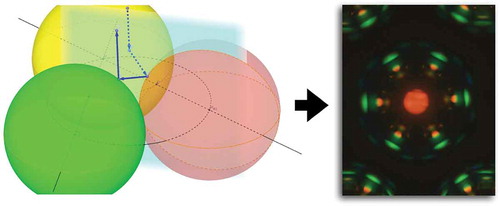
Figure 1. (Colour online) (a) Schematic drawing of the nested capillary set-up used for producing the CLC shells. The CLC is the middle fluid; the inner and outer fluids are isotropic aqueous solutions. (b) Shell production process captured by high-speed video camera. Scale bar is 200 m.

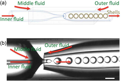
Figure 2. (Colour online) (a) Polarising microscopy image in transmission of hexagonally closed-packed CLC shells illuminated from below by linearly polarised white light and observed through a crossed analyser. Each shell diameter is about 250 m. (b) Schematic illustrations explaining the origin of the most fundamental reflection spots i (normal incidence reflection), ii (TIR-mediated communication) and iii (direct communication). For an introductory explanation of these communication pathways, see papers [24,25]. (c–j) Reflection polarising microscopy textures of a hexagonally close-packed CLC shell arrangement, illuminated with linearly polarised white light from above, with a field aperture that gradually increases from c–d to i–j. The original micrographs are in the left column (c, e, g, i) and the corresponding digitally enhanced images are shown in the right column (d, f, h, j), boosting the visibility of very weak reflections.

Figure 3. (Colour online) Ray path simulations for type i, ii and iii with expected colours emerging from the surface. The angle of incidence is the angle with which the illuminating rays impinge on the continuous phase surface, with respect to the vertical surface normal, and the angle is the corresponding angle of the rays that are reflected back to the microscope objective, defined with respect to the same vertical direction. One incident ray, corresponding to green direct communication of type iii, is drawn as a black arrow and several other possible reflections, corresponding to type i and type ii spots, are also shown. The Geogebra simulation can be accessed by the weblink https://ggbm.at/NceyNemH.

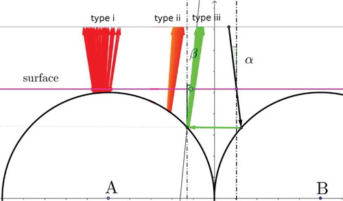
Figure 4. (Colour online) Ray path simulations for a type i spot with the expected colour emerging from the surface. The angle of incidence is varied from (black arrow in a) to (black arrow in c) with the reflected beams for all variations plotted simultaneously in all three panes. Measuring the diameter of the simulated spot in pane b () we find it to be about , where R is the outer radius of the shell, which matches the experimental data from Figure 2 quite well. The Geogebra simulation can be accessed by the weblink https://ggbm.at/NceyNemH.

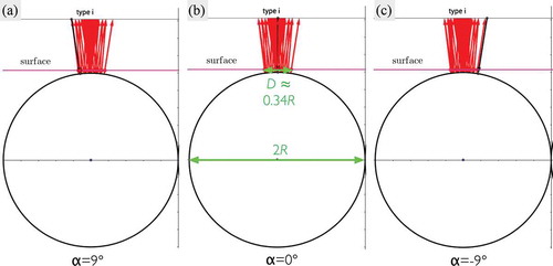
Figure 5. (Colour online) Ray path simulations for a type spot with the expected colour emerging from the surface. The left column assumes only surface reflection, but with incidence angle varying within the range allowed by the microscope illumination cone angle. While this reproduces the extension in space of the spot, it gives the wrong sequence of colours. The right column adds the possibility of below-surface reflection, and in this case the colour sequence as well as the extension in space are correct. Angle of incidence: ; Numerical aperture: ; Bragg reflection bandwidth: ; Radius of reflection surface: ; Wavelength for reflection of type ii: . The Geogebra simulation can be accessed by the weblink https://ggbm.at/NceyNemH.

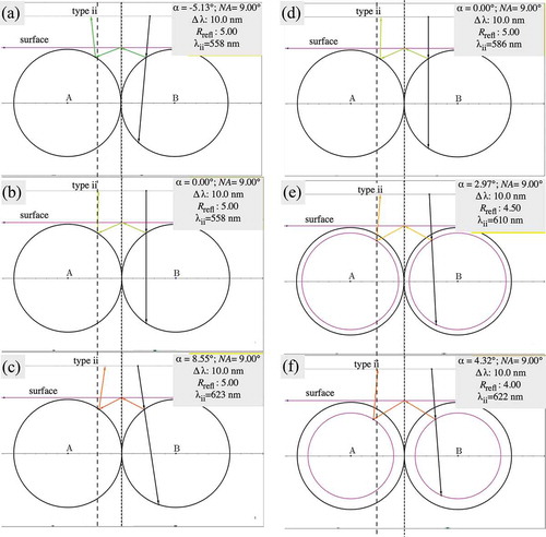
Figure 6. (Colour online) Ray path simulations for a type spot with the expected colour emerging from the surface. Two values of the incidence angle are shown, both within the opening angle of the microscope objective. The Geogebra simulation can be accessed by the weblink https://ggbm.at/NceyNemH.

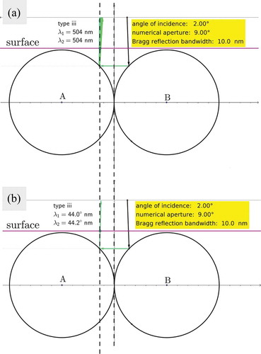
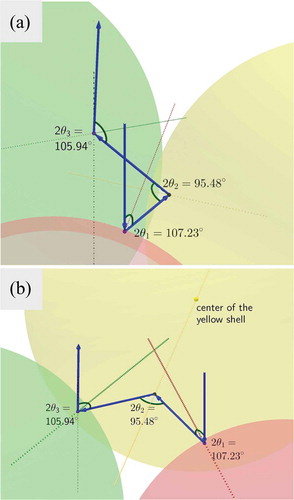
Figure 7. (Colour online) Three-shell communication responsible for blue reflections of type iv, viewed from two different angles. The central shell A is shown in red colour and two nearest neighbour B shells are shown in yellow and green, respectively. The angle of incidence is fixed at and for the depicted path . The angles of reflection (Bragg angles) within the path vary between 48° and 54°, corresponding to wavelengths , i.e. in the blue-violet range, requiring a large but reasonable bandwidth . The Geogebra simulation can be accessed by the weblink https://www.geogebra.org/m/cEsDHWfH.

Noh J, Liang H-L, Drevensek-Olenik I, et al. Tuneable multicoloured patterns from photonic cross communication between cholesteric liquid crystal droplets. J Mater Chem C. 2014;2(5):806–810.

 Web of Science ®Google Scholar

Noh J, Drevensek-Olenik I, Yamamoto J, et al. Dynamic and complex optical patterns from colloids of cholesteric liquid crystal droplets. In: Chien LC, Coles HJ, Kikuchi H, et al., editors. Proceedings of SPIE, emerging liquid crystal technologies X. San Francisco (CA): SPIE; 2015 Feb 9–13. p. X:93840T.

 Google Scholar