Considerations in the determination of orientational order parameters from X-ray scattering experiments

Figures & data

Figure 1. (Colour online) Schematic representation of an experimental X-ray scattering experiment for magnetically aligned nematic samples.

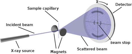
Figure 2. Unmodified X-ray scattering patterns obtained from (a) 5CB, (b) 6CB, (c) 7CB, (d) 8CB recorded at the lowest respective reduced temperature used for each sample (listed in the Supporting Information).

Figure 3. Background-subtracted X-ray scattering patterns obtained from (a) 5CB, (b) 6CB, (c) 7CB, (d) 8CB recorded at the lowest respective reduced temperature used for each sample (listed in the Supporting Information).

Figure 4. (Colour online) Integrated intensity profiles, I(χ), obtained from the background-subtracted experimental X-ray scattering patterns of 5CB, 6CB, 7CB and 8CB. Curves are coloured according to temperature (listed in the Supporting Information) from the highest (red) to the lowest (blue), and arrows show the direction of change on cooling.

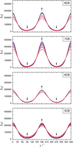
Figure 5. Background-subtracted X-ray scattering pattern of 5CB showing the wide-angle integration limits (white rings) and the regions used to estimate the baseline offset (grey-shaded areas). The horizontal white line corresponds to χ = 0°.

Figure 6. (Colour online) Order parameters, ⟨P₂⟩ and ⟨P₄⟩, of 5CB, 6CB, 7CB and 8CB obtained from background-subtracted, baseline-corrected scattering patterns recorded at the lowest respective reduced temperatures using the LM method (dashed lines) and the Kratky method truncating the expansion at different values of L (circles).

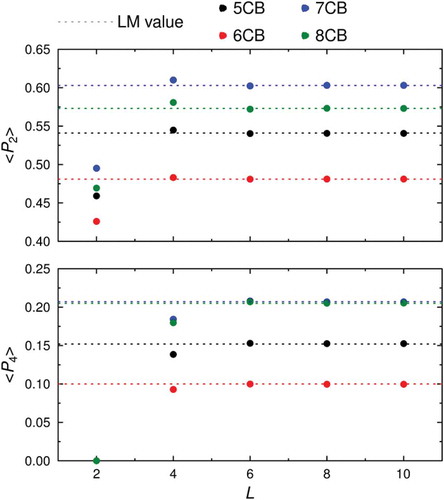
Figure 7. (Colour online) Experimental second-rank order parameters, ⟨P₂⟩, for 5CB, 6CB, 7CB and 8CB, determined from integrated intensity profiles from background-subtracted and either baseline-offset or zero-offset scattering patterns. The vertical dashed line denotes the N-SmA transition of 8CB [57].

Figure 8. (Colour online) Experimental fourth-rank order parameters, ⟨P₄⟩, for 5CB, 6CB, 7CB and 8CB, determined from integrated intensity profiles from background-subtracted and either baseline-offset or zero-offset scattering patterns. The vertical dashed line denotes the N-SmA transition of 8CB [57].

Figure 9. (Colour online) Comparison of second-rank order parameters, ⟨P₂⟩, of 5CB obtained from background-subtracted and baseline-offset data using the Kratky/LM method plotted against reduced temperature from this work, and from a range of reported values.

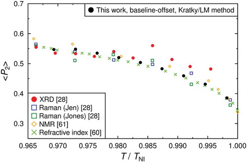
Figure 10. (Colour online) Comparison of fourth-rank order parameters, ⟨P₄⟩, of 5CB obtained from background-subtracted and baseline-offset data using the Kratky/LM method plotted against reduced temperature from this work, and from a range of reported values.

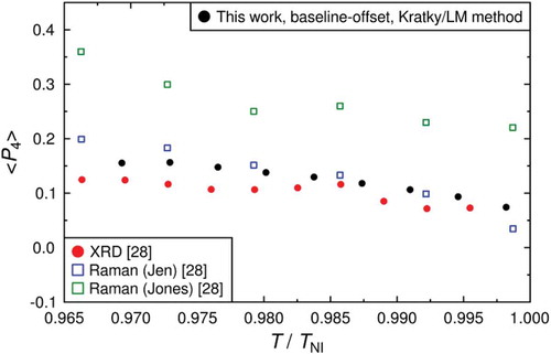
Figure 11. (Colour online) Maximum entropy orientational distributions (top) and sugar-loaf and diffuse-cone orientational distributions (bottom) with associated order parameters, ⟨P₂⟩ and ⟨P₄⟩.

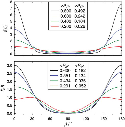
Figure 12. (Colour online) Calculated intensity profiles, I(χ), obtained from the maximum entropy distributions (top) and the sugar-loaf and diffuse-cone distributions (bottom) by numerical integration of Equation (5). The curves are coloured to match the distributions given in Figure 11.

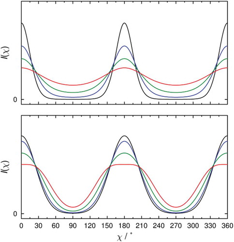
Table 1. Values, differences, Δ, and percentage differences, Δ(%), of the true order parameters, ⟨P₂⟩ and ⟨P₄⟩, of the maximum-entropy distributions shown in Figure 11 and those determined using the LN method.

⟨P2⟩				⟨P4⟩
True	LN	Δ	Δ(%)	True	LN	Δ	Δ(%)
0.800	0.796	−0.004	−0.5	0.492	0.488	−0.004	−0.8
0.600	0.572	−0.028	−4.7	0.242	0.228	−0.014	−5.8
0.400	0.355	−0.045	−11.3	0.104	0.090	−0.014	−13.5
0.200	0.163	−0.037	−18.5	0.026	0.021	−0.005	−19.2

Table 2. Values, differences, Δ, and percentage differences, Δ(%), of the true order parameters, ⟨P₂⟩ and ⟨P₄⟩, of the diffuse-cone-like distributions shown in Figure 11 and those determined using the LN method.

⟨P2⟩				⟨P4⟩
True	LN	Δ	Δ(%)	True	LN	Δ	Δ(%)
0.600	0.594	−0.006	−1.0	0.182	0.178	−0.004	−2.2
0.551	0.543	−0.008	−1.5	0.134	0.130	−0.004	−3.0
0.434	0.423	−0.011	−2.5	0.035	0.034	−0.001	−2.9
0.291	0.282	−0.009	−3.1	−0.052	−0.042	0.010	19.2

Table 3. Values, differences, Δ, and percentage differences of the true order parameters, ⟨P₂⟩ and ⟨P₄⟩, of the maximum-entropy distributions shown in Figure 11 and those determined using the LM method after applying a zero-offset to the calculated scattering intensity profiles.

⟨P2⟩				⟨P4⟩
True	Zero-offset	Δ	Δ(%)	True	Zero-offset	Δ	Δ(%)
0.800	0.806	0.006	0.8	0.492	0.495	0.003	0.6
0.600	0.658	0.058	9.7	0.242	0.266	0.024	9.9
0.400	0.558	0.158	39.5	0.104	0.145	0.041	39.4
0.200	0.476	0.276	138.0	0.026	0.063	0.037	142.3

Table 4. Values, differences, Δ, and percentage differences of the true order parameters, ⟨P₂⟩ and ⟨P₄⟩, of the diffuse-cone-like distributions shown in Figure 11 and those determined using the LM method after applying a zero-offset to the calculated scattering intensity profiles.

⟨P2⟩				⟨P4⟩
True	Zero-offset	Δ	Δ(%)	True	Zero-offset	Δ	Δ(%)
0.600	0.606	0.006	1.0	0.182	0.184	0.002	1.1
0.551	0.564	0.013	2.4	0.134	0.138	0.004	3.0
0.434	0.466	0.032	7.4	0.035	0.037	0.002	5.7
0.291	0.350	0.059	20.3	−0.052	−0.062	−0.010	19.2

Hird M. Physical properties of liquid crystals: nematics. Dunmur DA, Fukuda A, Luckhurst GR, editors.London: IET;2001.p. 3–16.

 Google Scholar