Rapid thickness mapping of free-standing smectic films using colour information of reflected light

Figures & data

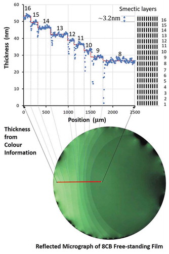
Figure 1. Multiple reflection from the free-standing film in air

Figure 2. (Colour online) (a) Simulated RGB colour coordinates for the three-colour light source emitting at 650 nm, 550 nm and 450 nm for thickness $h$ from 0–600 nm, and (b) the colour of reflection. The refractive index of the film is $n=$1.8

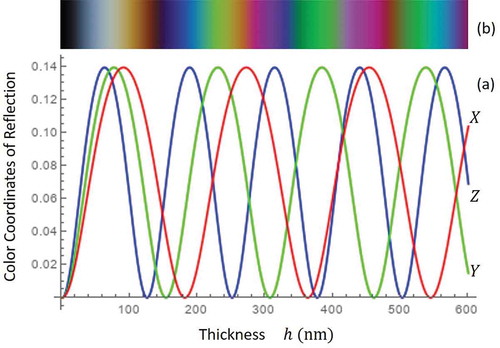
Figure 3. (Colour online) (a) Normalised colour coordinates for simulated reflections for the three-colour light source, and (b) the pure colour of reflection as a function of the thickness

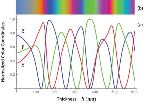
Figure 4. (Colour online) Normalised colour coordinates plotted on the unit sphere colour space (colour quadrant). The solid line shows the trajectory of $\left(\bar{X}\left(h\right),\bar{Y}\left(h\right),\bar{Z}\left(h\right)\right)$ for $h=$0 – 600 nm. Neighbouring dots are separated by 10 nm

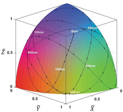
Figure 5. (Colour online) Arc length $\delta s$ per 1 nm of thickness change for the three-colour light source. (a) $h=$0 – 600 nm. (b) Magnified view of (a) for $h=$0 – 100 nm

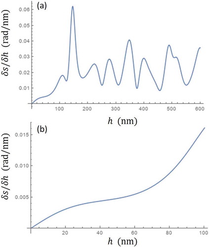
Figure 6. (Colour online) Colour-thickness trajectory on the colour quadrant for the dispersive refractive index (White line). Black line is the trajectory for a constant refractive index

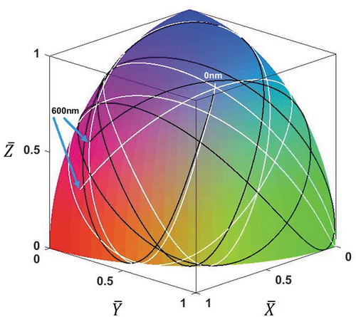
Figure 7. (Colour online) The optical setup for the thickness measurement system based on a stereomicroscope. The free-standing film is inside a closed chamber with two tilted glass windows

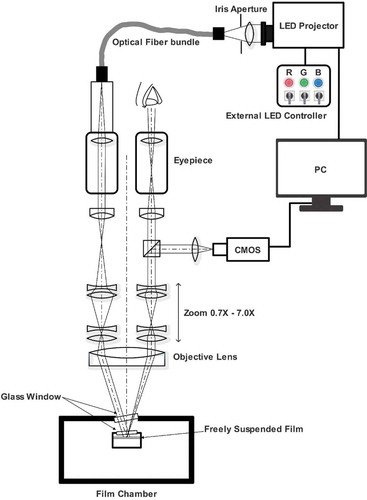
Figure 8. (Colour online) Reference images, cross sectional intensity profiles and colour maps at 0.7X magnification [(a), (b) & (c)] and at 7.0X [(d), (e) & (f)]. A plain silver mirror was set in place of the film. The intensity profiles in (b) & (e) correspond to the cross section in (a) & (b) indicated by broken white lines running the centre

Figure 9. (Colour online) The illumination spectrum $I\left(\lambda \right)$ at the camera port, corrected for a hypothetical perfect mirror reflection (Red line). The black line shows the spectrum observed immediately from the LED projector. The difference is ascribed to loss due to the microscope optics

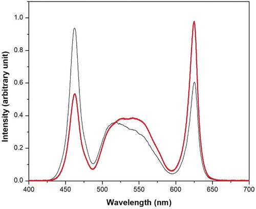
Figure 10. (Colour online) (a) Optical setup for measuring the colour filter transmission functions of the CMOS camera. (b) Transmission functions for Red, Blue and Green colour filters of the camera

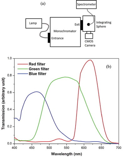
Figure 11. (Colour online) Colour-thickness trajectory on the colour quadrant for observation of free-standing films of 4-octyl-4ʹ-cyanobiphenyl (8CB) in the present optical setup. The black line and dots indicate the trajectory without adjustment($\alpha =0$). The white line and dots are for the case with $\alpha =1.0$. Dots are plotted every 10 nm

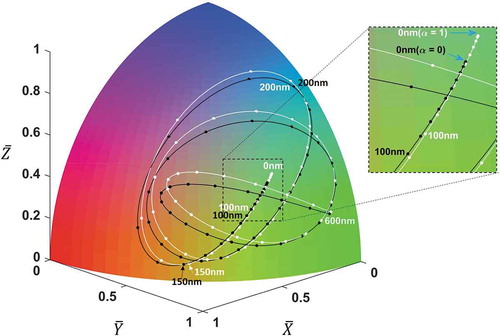
Figure 12. (Colour online) Graphical User Interface (GUI) of the MATLAB software for thickness mapping of free-standing films. Top right is the real time image of the film, and the bottom right displays the saved image to be analysed. The corresponding colour map on the colour quadrant is shown on the left side with the thickness versus the square root intensity plot (to the right) and the cross sectional thickness profile (centre left) along the red line drawn manually on the target image on the bottom right

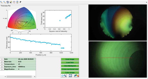
Figure 13. (Colour online) (a) Raw image of a free-standing smectic film of 8CB captured at 0.7X magnification and 40 ms exposure time. (b) The colour coordinates along the cross section (white broken line in (a)) plotted as semi-transparent white dots on the colour quadrant along with the colour-thickness trajectory for $\alpha =1.0$

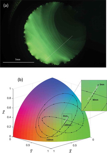
Figure 14. Pixel-wise film thickness plotted against the square root of the pixel-wise reflectivity $R_F$ for $\alpha =1.0$

Figure 15. (Colour online) Distribution of pixel-wise thicknesses along the 800$\mu$m-long cross section (broken white line in the inset) indicated as a histogram of pixel counts per 0.1 nm thickness window. The free-standing film of 8CB was equilibrated for over 24 hours to be uniform in thickness, and imaged at 3.0X magnification for 0.42 sec exposure. The average of 10 images was taken to enhance S/N ratio. The brown line shows the best fit Gaussian

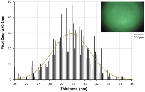
Figure 16. (Colour online) (a) Raw image of a free-standing smectic film of 8CB captured at 2.0X magnification and 40 ms exposure time. (b) The colour coordinates of whole pixels plotted as semi-transparent white dots on the colour quadrant along with the colour trajectory. All pixels from the entire image with the intensity higher than 20% of the peak intensity are selected

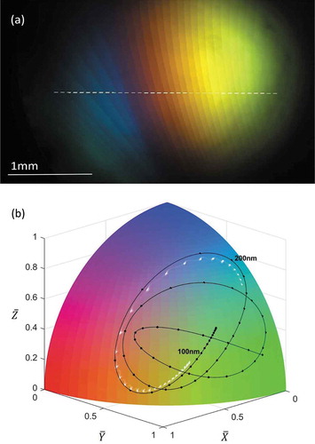
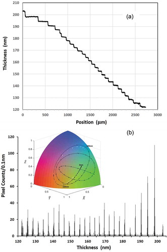
Figure 17. (Colour online) (a) Cross sectional thickness profile along the white broken line in Fig.16(a). (b) Histogram of pixel counts per 0.1 nm window of thickness for the cross section; the inset shows colour coordinates along the cross section plotted on the colour quadrant. The largest and smallest thickness peaks are located at 203.0$\pm$0.2 nm and 122.3$\pm$0.3 nm, respectively, and there are 27 layers. The smectic layer thickness (average spacing between neighbouring peaks) is evaluted to be 3.10$\pm$0.02 nm