Rapid thickness mapping of free-standing smectic films using colour information of reflected light II: real-time areal mapping using lookup table scheme

Figures & data

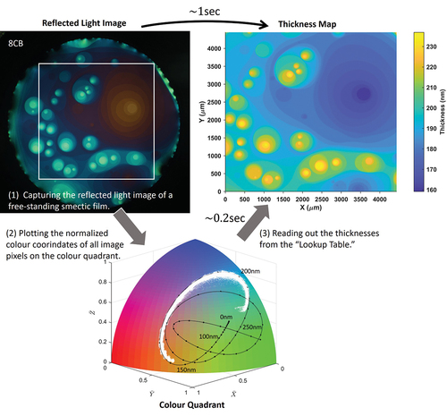
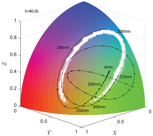
Figure 1. (Colour online) Colour quadrant and the theoretical thickness-colour trajectory for 8CB(4-octyl-4ʹ-cyanobiphenyl) from 0 nm to 600 nm thickness. $O_z$ stands for the 0-thickness point.

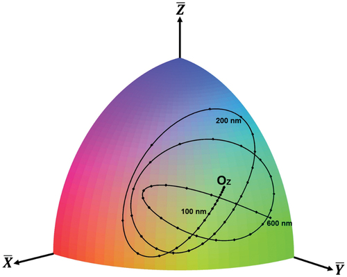
Figure 2. (Colour online) Construct of modified hierarchical triangular partition of the colour quadrant. The equilateral triangle $ABC$ is one of the faces of octahedron, from which the partitioning starts. $O_z$ is the 0-thickness point on the colour quadrant, and the radial line $O_0{O}_z$ is extended by a factor of $\alpha$ to the point $O$. An arbitrary point $P$ on the colour quadrant is radially projected to $Q$, which is on either of the three triangles $OAB$, $OBC$ and $OCA$. In this example, the point $Q$ is on $OAB$, and the line passing $O$ and $Q$ intersects the line $AB$ at the point $E$.

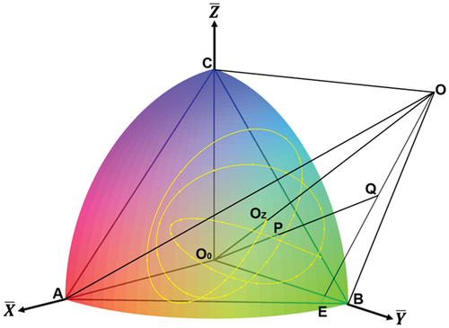
Figure 3. (Colour online) Partitioning the equilateral triangular pyramid $ABCO$ covering the entire colour quadrant. Each face is partitioned into identically shaped child triangles. In this example, $N=10$, and each of $OAB,OBC$and $OCA$ contains $N^2=100$ child triangles.

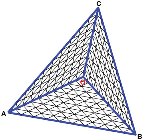
Figure 4. (Colour online) The spherical triangular mesh partitioning the colour quadrant. The red dots on the trajectory indicate 10 nm differences of the thickness. Here we have used $\alpha =4$ and $N=10$ to make the partitions clearly visible relative to the 0-thickness point.

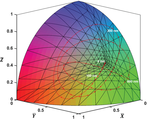
Figure 5. (Colour online) Two types of child triangles and the schematic illustration of indexing. $N=10$. The white triangle with a black dot is indexed as $\left(l,m,n\right)=\left(7,7,8\right)$ following the blue arrows from the edges. Note that $l+m+n=22=2N+2$.

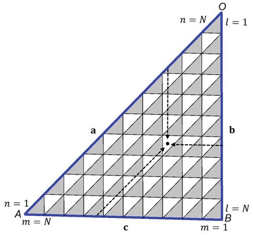
Figure 6. Schematic summary of indexing, lookup table and lookup steps of data points. The lookup table $\left(k\right)$ is generated following the upper steps from the partitioning of the mother triangles. The colour data point $\mathbf{P}$ is analysed following the lower steps to obtain the corresponding linear index $k$, which is looked up in the lookup table to obtain the thickness $h\left(\mathbf{P}\right)$.

Figure 7. (Colour online) (a) Reflected image of free-standing smectic film at 4.0$\times$ magnification. (b) Histogram of thickness for 0.1 nm for nearly one million pixels within the rectangular region in (a). The average layer thickness calculated from this result is 3.17 ± 0.01 nm. (c) Top view of the thickness profile for the selected rectangular region in (a). (d) 3D view of the thickness profile.

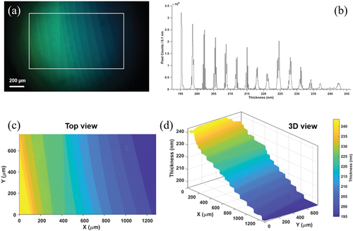
Figure 8. CPU execution time for thickness calculation as a function of the number of data points.

Figure 9. (Colour online) Series of snapshots extracted from the AVI video of free-standing smectic film captured in the free-run mode at 0.7$\times$ magnification: (a) t = 5.25 s, (d) t = 10.03 s, (g) t = 18.68 s, and (j) t = 33.81 s. Top view (b, e, h, and k) and 3D view (c, f, i, and l) of the thickness map for images on the left. The full video is available as Supplemental Material.

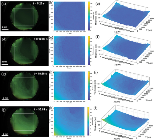
Figure 10. (Colour online) Series of snapshots extracted from the AVI video of relatively thick free-standing smectic film immediately after the sudden deflation. Captured in the free-run mode at 1.13 fps. (a) & (b) t = 40.0 s, (c) & (d) t = 92.7 s, (e) & (f) t = 90.2 s, and (g) & (h) t = 182.4 s. (a, c, e, g) Reflected microscopic images. (b, d, f, h) Top views of thickness map. The full video is available as Supplemental Material.

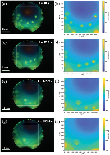
Figure 11. (Colour online) Distribution of data points (white dots) on the colour quadrant for the free-standing film shown in Figure 10(a) with t = 40.0s.