Connectome analysis for pre-operative brain mapping in neurosurgery

Figures & data

Table 1. Demographic information.

Patient	Age	Pre-operative examination	Pathology	Operation	Tumour location	Tumour volume (mm^3)
1	64	Left pronator drift	Glioblastoma	Complete resection	Right superior parietal lobule	35,736
2	73	Intact	Glioblastoma	Complete resection	Right inferior parietal lobule to occipital pole	86,296
3	79	Hemianopia	Glioblastoma	Complete resection	Right inferior occipital lobe	46,232
4	76	Left hemiparesis	Glioblastoma	Biopsy	Right superior para-central lobule	59,304
5	36	Left hemiparesis	Glioblastoma	Complete resection	Right post-central gyrus and supramarginal gyrus	51,544

Figure 1. Connectome construction. Methods for performing a connectome analysis using resting-state fMRI data as an example, but similar methods can be applied to data acquired from DTI or EEG/MEG. Initially, a template is chosen to divide the brain into different regions (known as parcels) that form the network nodes. These nodes are used to form the rows and columns of a matrix. Entries of the matrix represent edges between each of the nodes and are formed by recording a measure of statistical dependency (such the Pearson correlation co-efficient) between the resting-state fMRI time series of each node. This correlation matrix can then be thresholded and binarised to form an adjacency matrix, although weighted and fully connected matrices (without thresholding) are also possible. Finally, the co-ordinates of each parcel are used to display the node location onto a surface reconstruction of the brain, with edges representing functional connections.

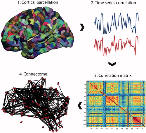
Table 2. Definitions of network measures.

Measure	Definition
Centrality	How important a given node’s features are to the overall network
Degree	The number of connections of a node
Efficiency	The inverse of path length (which accounts for disconnected nodes and weights more towards short edges). Can be local (based on a nodes community) or global
Clustering co-efficient, γ	The clustering co-efficient measure of local cliques or nodes whose neighbours are also neighbours of each other and is a measure of network segregation. This can be expressed as a ratio of that from a corresponding random network (‘normalized clustering co-efficient’)
Giant component	Largest connected cluster of nodes in a network
Hub	Nodes that form a key component of the overall network structure e.g. they have high degree, high centrality, or short path length to other nodes
Information centrality	Percentage change in global efficiency due to removal of a single node
Path length, λ	Path length is the number of discrete steps between nodes that are required to complete a journey from one node to another and is a measure of network integration. This can be expressed as a ratio of that from a corresponding random network (‘normalized path length’)
Random error	Removing nodes at random and measuring the change in network properties (e.g. size of the giant component or efficiency)
Resilience	The ability of a network to recovery from removal of specific components (nodes or edges). A network that is highly resilient will demonstrate little change in its graph theory measures after removing node(s) or edges(s). This definition is similar to robustness but implies a dynamic reparative process such as plasticity
Robustness	The ability of a network to maintain its typical graph theory characteristics after removal of specific node(s) or edge(s) i.e. a network that is robust will tend not to change much after removal of specific components
Small world, δ	A measure of simultaneous clustering (network segregation) and short path length (network integration) formed by network short-cuts. Typically defined as γ/λ >1
Targeted attack	Removing nodes based on a ranking of network features (e.g. degree, centrality, or clustering)

Figure 2. Effects of thresholding on network degree. Increasing the cut-off of the correlation threshold results in a reduction in the number of edges that survive thresholding in the resulting matrix. The straight black line represents the minimum mean degree for small world networks (n*log(n) = 9.5). The point of intersection of the wavelet scale degree with this line is used as the threshold to form the binary network used for further analysis. Wavelet scales 4 and 5 were not able to produce a matrix of the required mean degree at any threshold and were, therefore, not studied further.

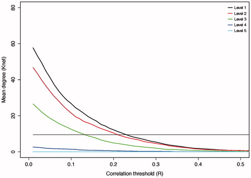
Table 3. Small world features for group networks per wavelet scale.

Scale	Hz	r	R	Lnet	Cnet	λ	γ	δ
1	0.10–0.20	0.28	0.23	3.53	0.54	1.50	1.83	1.22
2	0.05–0.10	0.35	0.21	2.72	0.56	1.17	1.94	1.65
3	0.03–0.05	0.41	0.13	2.99	0.61	1.29	1.96	1.51

Increasing wavelet scale represents decreasing frequency. Wavelet scales 4 and 5 are not shown as they did not produce the required mean degree for a small world network (see Figure 3). r is the mean correlation of the scale; R is the correlation threshold to form the adjacency matrix; L_net is the mean path length; C_net is the mean clustering co-efficient; λ is the ratio of path length to that of a corresponding random network; γ is the ratio of clustering co-efficient to that of a corresponding random network; δ, small world measure (δ = γ/λ).

Figure 3. The connectome in glioblastoma. A sagittal view of an individual patient’s connectome at wavelet scale 2. Nodes are coloured according to their anatomical module (e.g. frontal, central, parietal, etc.) and their size is proportional to their degree. Connections (or edges) are presented in grey and represent the binary entries of the adjacency matrix. Locations are based on the co-ordinates of their original parcels and projected onto a surface reconstruction in MNI space.

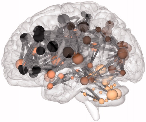
Table 4. Complete network measures.

Side	Parcel abbreviation	Degree	Clustering	Path length	Information centrality
l	MCIN	31	0.51	2.15	−3.43
l	PQ	31	0.35	1.94	−3.59
r	F1	30	0.41	1.99	−3.26
r	MCIN	28	0.53	2.23	−3.09
r	F2	28	0.51	2.18	−3.10
l	SMA	27	0.62	2.25	−3.01
l	T1	26	0.55	2.45	−2.84
r	T1	26	0.58	2.45	−2.81
r	PQ	25	0.38	2.11	−3.34
l	SMG	24	0.66	2.32	−2.85
l	F2	24	0.46	2.13	−4.44
l	PRE	23	0.68	2.29	−2.82
l	F3OP	23	0.69	2.40	−2.74
r	SMA	23	0.72	2.39	−2.76
r	F3T	22	0.61	2.37	−2.79
l	F1	22	0.49	2.09	−2.96
l	POST	22	0.69	2.25	−2.83
r	POST	22	0.61	2.24	−2.97
r	F3OP	21	0.78	2.38	−2.72
r	SMG	21	0.66	2.32	−2.77
l	IN	20	0.64	2.54	−2.62
l	V1	20	0.46	2.24	−2.86
l	RO	19	0.77	2.59	−2.55
r	PRE	19	0.73	2.30	−2.70
r	F1M	19	0.39	2.29	−3.00
l	O2	19	0.51	2.37	−2.78
l	F3O	18	0.53	2.43	−2.63
l	T2	18	0.56	2.32	−2.74
l	F1M	17	0.38	2.34	−2.80
l	LING	17	0.47	2.24	−3.40
r	RO	15	0.72	2.64	−3.94
l	PCL	15	0.81	2.49	−2.52
l	Q	14	0.67	2.31	−2.59
r	Q	14	0.69	2.52	−2.44
l	O3	14	0.66	2.41	−2.52
r	T2	14	0.44	2.37	−2.87
r	LING	13	0.74	2.49	−2.42
l	P2	13	0.51	2.43	−2.50
r	IN	12	0.62	2.85	−2.29
l	PCIN	12	0.56	2.43	−2.51
r	V1	12	0.82	2.54	−2.38
r	O3	12	0.73	2.64	−2.31
l	P1	11	0.56	2.44	−2.47
r	P2	11	0.64	2.52	−2.41
r	CVCU	10	0.44	2.37	−4.03
l	O1	10	0.53	2.91	−3.51
r	FUSI	10	0.38	2.83	−3.76
r	PCL	10	1.00	2.74	−2.25
l	F3T	9	0.86	2.68	−2.28
l	AG	9	0.64	2.57	−2.32
r	AG	9	0.69	2.61	−2.31
l	T1P	9	0.42	2.89	−2.42
l	ACIN	8	0.46	2.85	−2.21
r	ACIN	7	0.52	2.89	−2.15
r	O2	7	0.86	2.84	−2.08
l	HES	7	0.95	2.97	−2.09
r	CHS	6	0.27	3.46	−2.16
r	F1MO	6	0.67	3.10	−1.95
l	FUSI	6	0.67	2.89	−2.03
r	P1	6	0.67	2.84	−2.06
r	T1P	6	0.40	3.25	−1.94
l	CHCU	6	0.40	3.05	−3.21
l	CHS	6	0.27	2.93	−2.64
r	CVD	5	0.40	3.07	−3.15
r	F3O	5	0.50	3.00	−2.01
r	GR	5	0.30	3.13	−2.21
l	F1MO	4	0.50	3.20	−1.85
r	CAU	4	0.33	1.33	−0.50
r	T2P	4	0.33	3.25	−1.84
r	CHCU	4	0.33	3.13	−3.06
r	F2O	3	0.67	3.94	−1.45
r	PCIN	3	1.00	2.87	−1.98
l	HIP	3	0.67	1.25	−0.20
l	PHIP	3	0.33	1.25	−0.28
r	PHIP	3	0.67	1.25	−0.20
l	F1O	3	0.67	3.94	−1.45
r	F1O	3	0.33	4.05	−1.51
l	PUT	3	0.33	1.67	−0.36
l	THA	3	0.33	1.67	−0.36
l	F2O	3	0.33	3.05	−2.44
l	CHSS	3	0.00	3.83	−2.58
r	CHSS	3	0.00	4.36	−3.17
l	GR	2	0.00	4.09	−1.40
r	HIP	2	1.00	1.75	−0.16
r	O1	2	1.00	3.75	−1.53
l	CAU	2	1.00	1.83	−0.22
r	PUT	2	1.00	1.83	−0.22
l	T2P	2	1.00	3.79	−1.54
r	CHIS	2	0.00	5.32	−1.94
l	CHG	1	−1.00	1.00	−0.06
r	CHG	1	−1.00	6.31	−0.89
l	CHB	1	−1.00	1.00	−0.06
r	CVT	1	−1.00	4.06	−1.34
l	AMYG	1	−1.00	2.00	−0.13
l	PAL	1	−1.00	2.50	−0.17
r	THA	1	−1.00	2.50	−0.17
r	HES	1	−1.00	3.63	−1.57
l	T3	1	−1.00	3.90	−1.44
r	T3	1	−1.00	3.82	−1.46
l	CHIS	1	−1.00	4.82	−1.14
l	CHCL	1	−1.00	4.03	−1.36
r	CHCL	1	−1.00	4.11	−1.32
r	CHB	0	−1.00	−1.00	0.00
l	CHT	0	−1.00	−1.00	0.00
r	CHT	0	−1.00	−1.00	0.00
l	CHF	0	−1.00	−1.00	0.00
r	CHF	0	−1.00	−1.00	0.00
l	CVL	0	−1.00	−1.00	0.00
l	CVCL	0	−1.00	−1.00	0.00
r	CVP	0	−1.00	−1.00	0.00
l	CVU	0	−1.00	−1.00	0.00
l	CVN	0	−1.00	−1.00	0.00
l	OC	0	−1.00	−1.00	0.00
r	OC	0	−1.00	−1.00	0.00
r	AMYG	0	−1.00	−1.00	0.00
r	PAL	0	−1.00	−1.00	0.00

Network measures are shown for all parcels in order of descending degree. Note that for the last parcels where the degree is the lowest the parcel can be outside of the main giant component of the network making clustering and path length values inaccurate. Parcel abbreviations are the same as in Figure 7. Regions are ranked in order of decreasing degree.

Figure 4. Degree distribution. (A) The histogram for the group network node degrees. The majority of nodes are of low degree (<5) while the maximum degree extends above 30 (although few nodes have this degree). (B) The group network degree distribution is compared to that from simulated networks with either an exponential, power law, or exponentially truncated power law degree distribution. The best fit determined using Akaite Information Criteria was with the exponentially truncated power law degree distribution.

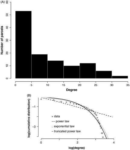
Figure 5. Random error and targeted attack. The change in the size of the network giant component (top row) or efficiency (bottom row) due to either random error (left column) or targeted attack based on degree centrality (right column). Changes are relative to the values for the intact network. All networks are approximately equally affected by random error. However, targeted attack reveals vulnerability of the scale free network, while the brain network is of intermediate vulnerability between the scale-free and random networks. Horizontal axis values are the proportion of nodes removed and vertical axis values are scaled to maximum. Solid line = brain networks, dotted line = simulated scale-free networks, dashed line = simulated random networks

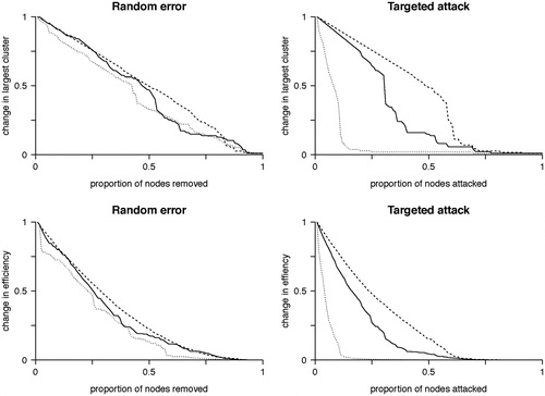
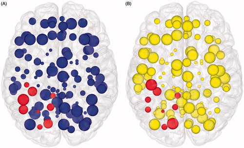
Figure 6. Brain mapping with graph theory network measures. Axial view of node features displayed in cortical surface reconstructions. (A) Node size is proportional to clustering co-efficient. (B) Node size is proportional to information centrality. In both figures, those nodes that are spatially adjacent to the tumour are highlighted. Network edges are removed to focus on the node features. If one were to use this information for pre-surgical planning, purposefully sacrificing selected smaller nodes to allow an extended surgical resection could be seen as having a minimal effect on overall network efficiency (and, therefore, by extrapolation on higher cognitive features such as intelligence). However, inadvertently affecting too many of larger nodes would be expected to have a disproportionate effect on overall network efficiency, and, therefore, should be avoided.