Relationships between diatoms and tidal environments in Oregon and Washington, USA

Figures & data

Fig. 1. Location of study sites (filled circles) along the coast of Oregon and Washington in the northwestern United States. Triangles indicate tide gauge stations (labeled in gray).

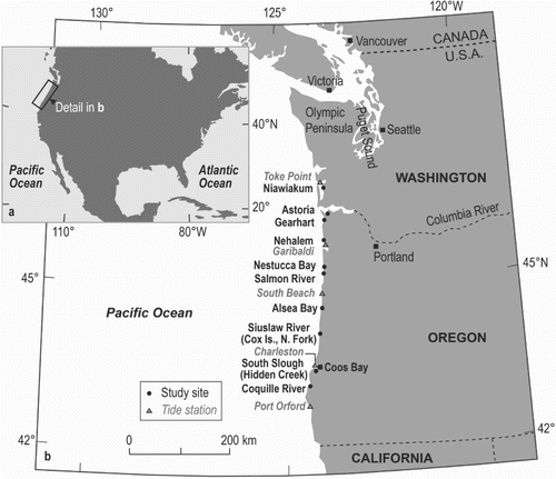
Fig. 3. Data analysis of diatom assemblages at the Salmon River (Oregon, USA). (a) A diagram of the studied transect at the Salmon River. Vertical and horizontal axes represent elevation (m) relative to MTL and distance (m), respectively. Surface samples were collected across four recognizable environmental zones: tidal flat, low marsh, middle marsh, high marsh, and supratidal. Dominant vascular plant species are listed for zones. (b) Changes in abundance (%) of dominant diatom species along the transect. (c) Result of agglomerative hierarchical cluster analysis. (d) DCA results for diatom distribution in the 14 surface samples.

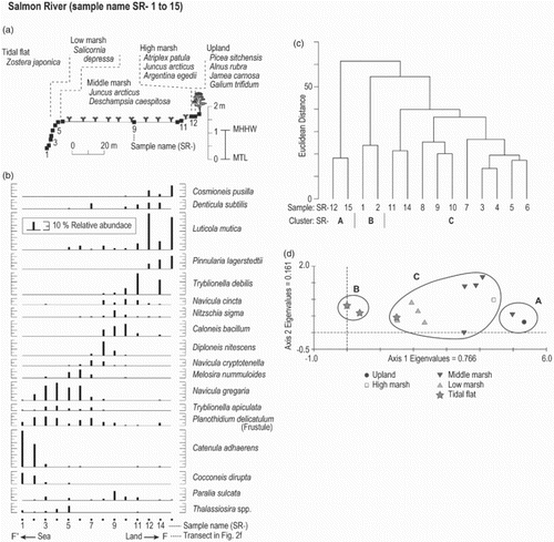
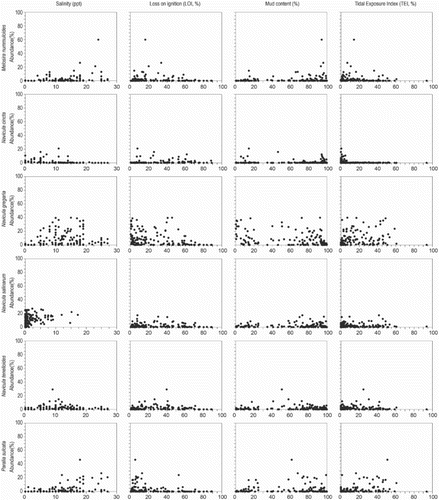
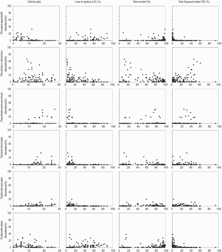
Fig. 6. Results of detrended correspondence analysis (DCA) showing patterns of variation in diatom sample assemblages for the combined regional dataset. The environmental variables were added as supplementary variables. Numbers of samples at each site are shown in Table A1.

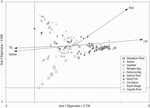
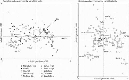
Fig. 7. Results of canonical correspondence analysis (CCA) for the combined regional dataset: (Left) sample-environment bi-plots. (Right) species-environment bi-plots. Species abbreviations are as follows: Cosmioneis pusilla (COSPU), Diploneis didyma (DIPDYD), Eunotia praerupta (EUPRA), Gyrosigma eximium (GYEX), Melosira moniliformis (MEMO), Navicula cancellata (NACAN), Navicula cincta (NACI), Navicula gregaria (NAGRE), Navicula palpebralis (NAPAL), Navicula salinicola (NASALI), Navicula salinarum (NASAL), Navicula slesvicensis (NASLE), Paralia sulcata (PASU), Pinnularia borealis (PINBOR), Pinnularia lagerstedtii (PINLAG), and Tryblionella salinarum (TRYSA).

Table 1. Summary of CCA results for combined regional diatom dataset (species with maximum relative abundance greater than 5%).

Axes	1	2	3	4	Total inertia
Eigenvalues	0.612	0.312	0.263	0.152	12.587
Species-environment correlations	0.930	0.807	0.831	0.701
Cumulative percentage variance
of species data	4.9	7.3	9.4	10.6
of species-environment relation	45.7	69.0	88.6	100
Sum of all eigenvalues					12.587
Sum of all canonical eigenvalues					1.339

Table 2. Environmental variables selected using manual forward selection within CANOCO.

Variable	% of variance	F-value	p-value
Explained
Salinity	2.2% (20.1%)	3.268	0.001
Loss on ignition (LOI weight %)	1.9% (17.9%)	6.158	0.001
Mud content (weight %)	2.4% (22.6%)	3.530	0.001
Tidal exposure index (TEI %)	1.8% (17.0%)	2.682	0.001
Inter-correlation	2.3% (21.7%)
Unexplained	89.4%

Percentages of explained variables are calculated by variation partitioning of diatom species from the regional dataset (species with maximum relative abundance greater than 5%). The variances explained are their unique contributions. Numbers within parentheses represent contribution of explained variance among gradients.