Temporal changes in size distributions of the Southern Ocean diatom Fragilariopsis kerguelensis through high-throughput microscopy of sediment trap samples

Figures & data

Fig. 1. Map of the Southern Ocean with annual sea surface temperatures (SST; World Ocean Atlas 2013, Locarnini et al. 2013) showing the location of the 54°S station and the site of the European Iron Fertilization Experiment (EIFEX). Black line represents the position of the APF after Orsi et al. (1995).

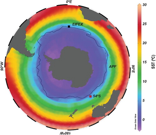
Fig. 2. Distributions of valve lengths and mixtures of univariate normal distributions for sampling year 2002/2003. Background colours red, green and blue depict phases 1, 2 and 3 explained in the text. Histograms show the distribution of measured valve lengths, the dashed curve their density estimate. Vertical dotted lines mark 31 µm, the size limit below which sexual reproduction can occur, and 75.5 µm, the minimal size of initial cells as reported by Assmy et al. (2006). Coloured curves depict the component normal distributions C1-Cn, the corresponding parameters are given in the graphs. Note that curves appearing in the same colour at different time points are not implied to correspond to the same cohort (colour online).

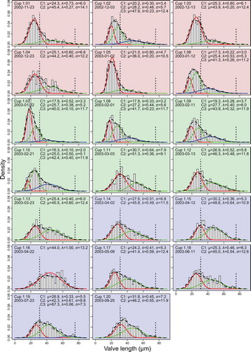
Fig. 3. Distributions of valve lengths and mixtures of univariate normal distributions for sampling year 2003/2004. Background colours red, green and blue depict phases 1, 2 and 3 explained in the text. Histograms show the distribution of measured valve lengths, the dashed curve their density estimate. Vertical dotted lines mark 31 µm, the size limit below which sexual reproduction can occur, and 75.5 µm, the minimal size of initial cells as reported by Assmy et al. (2006). Coloured curves depict the component normal distributions C1-Cn, the corresponding parameters are given in the graphs. Note that curves appearing in the same colour at different time points are not implied to correspond to the same cohort (colour online).

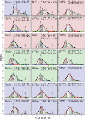
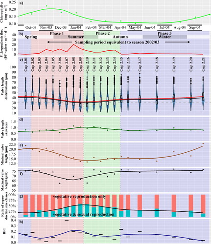
Fig. 4. Temporal variability during sampling year 2002/2003, x-axis refers to the middle day of sampling periods. (a) Chlorophyll-a concentration in the upper water column. (b–h) Sediment trap data from 800 m depth, for Fragilariopsis kerguelensis; depending on the sinking speed, the timeline is delayed by ca. 2–6 weeks compared to the chlorophyll data. Trend lines are derived by LOESS smoothing: (b) Valve flux. (c) Valve length. Blue violin plots depict the value distributions, box plots represent quartiles, red dots indicate the mean, black dots inside the boxplots the median. The dashed horizontal line depicts 31 µm, the size limit below which sexual reproduction can occur. (d) Seasonal changes in the valve length skewness. (e) Minimal valve length by 0.01 quantile. (f) Maximal valve length by 0.99 quantile. (g) Ratio of size fractions which are sexually inducible (that are capable of vegetative as well as sexual reproduction, with a valve length below 31 µm, highlighted in turquoise), respectively, capable of vegetative reproduction only (orange). (h) Relative frequency of valves within the initial cell size range (RFI), as an indicator for initial cells (colour online).

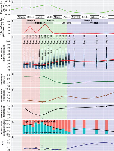
Fig. 5. Temporal variability during sampling year 2003/2004, x-axis refers to the middle day of sampling periods. (a) Chlorophyll-a concentration in the upper water column. (b–h) Sediment trap data from 800 m depth for Fragilariopsis kerguelensis; depending on the sinking speed, the timeline is delayed by ca. 2–6 weeks compared to the chlorophyll data. Trend lines are derived by LOESS smoothing: (b) Valve flux. (c) Valve length. Blue violin plots depict the value distributions, box plots represent quartiles, red dots indicate the mean, black dots inside the boxplots the median. The dashed horizontal line depicts 31 µm, the size limit below which sexual reproduction can occur. (d) Seasonal changes of the valve length skewness. (e) Minimal valve length by 0.01 quantile. (f) Maximal valve length by 0.99 quantile. (g) Ratio of size fractions which are sexually inducible (that are capable of vegetative as well as sexual reproduction, with a valve length below 31 µm, highlighted in turquoise), respectively, capable of vegetative reproduction only (orange). (h) Relative frequency of valves within the initial cell size range (RFI), as an indicator for initial cells (colour online).

Locarnini R.A., Mishonov A.V., Antonov J.I., Boyer T.P., Garcia H.E., Baranova O.K., Zweng M.M., Paver C.R., Reagan J.R. & Johnson D.R. 2013. World Ocean Atlas 2013. Volume 1, Temperature. S. Levitus, Ed., A. Mishonov Technical Ed.; NOAA Atlas NESDIS 73, 40 pp.

 Google Scholar

Orsi A.H., Whitworth III T. & Nowlin Jr W.D. 1995. On the meridional extent and fronts of the Antarctic Circumpolar Current. Deep Sea Research Part I: Oceanographic Research Papers 42: 641–673. doi: 10.1016/0967-0637(95)00021-W

 Web of Science ®Google Scholar

Assmy P., Henjes J., Smetacek V. & Montresor M. 2006. Auxospore formation by the silica-sinking, oceanic diatom Fragilariopsis kerguelensis (Bacillariophyceae). Journal of Phycology 42: 1002–1006. doi: 10.1111/j.1529-8817.2006.00260.x

 Web of Science ®Google Scholar