Is Anticipation Skill Learning Bayesian?

Figures & data

Figure 1. Anticipation accuracy scores for the pre- and posttests of the KIP-SPA and KIP-SPA group per condition (2080 R, 5050KIA, 5050KIP, 8020 L). Error bars represent standard error.

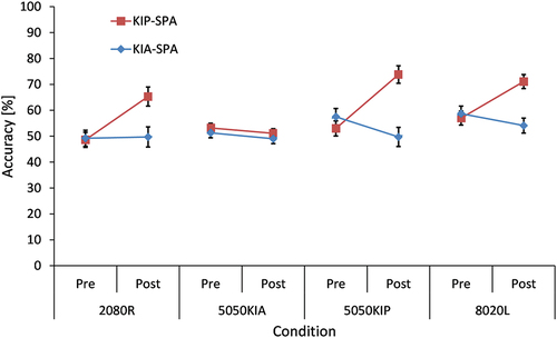
Figure 2. Anticipation accuracy scores of the KIP-SPA (red squares) and KIP-SPA (purple circles) group per each acquisition block (1–4). *indicates significant (p < .05) differences for the KIP-SPA group between the respective acquisition blocks. Error bars represent standard error.

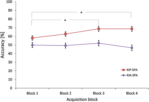
Figure 3. Effort scores of the KIP-SPA (red squares) and KIP-SPA (purple circles) group per each acquisition block (1–4). *indicates significant (p < .05) differences between the groups on the respective acquisition blocks. Error bars represent standard error.

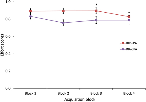
Figure 4. Anticipation accuracy scores for the pre- and posttests of the KIP-SPP and KIA-SPP group per condition (2080 R, 5050KIA, 5050KIP, 8020 L). Error bars represent standard error.

Figure 5. Response times [s] for the pre- and posttests of the KIP-SPP and KIA-SPP group per condition (2080 R, 5050KIA, 5050KIP, 8020 L). Error bars represent standard error.

Figure 6. Response accuracy for the left and right shot directions when learning with 2080 R and 8020 L shot probabilities during acquisition blocks 1–4. Error bars represent standard error.

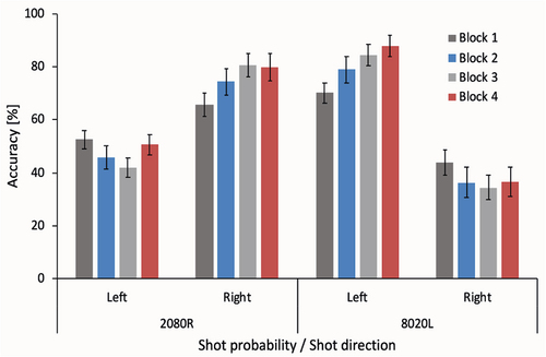
Figure 7. Response time for the left and right shot directions when learning with 2080 R and 8020 L shot probabilities during acquisition blocks 1–4. Error bars represent standard error.

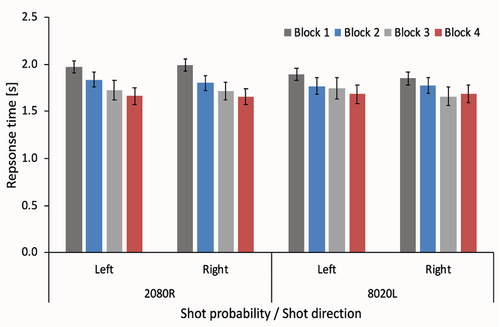
Figure 8. Rescaled odds ratio (bayes factor) comparing of each condition (2080 R, 5050KIA, 5050KIP, 8020 L) per each of the four groups (KIP-SPA, KIA-SPP, KIP-SPP, KIP-SPA) for the pre- and post- tests. For ease of interpretation results have been rescaled such that equi-probable responses have a value of 0 and both positive and negative integers represent the number of times more likely a congruent (positive) and incongruent (negative) response was seen. Error bars represent standard error.

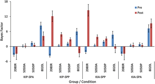
Figure 9. Rescaled odds ratio (Bayes Factor) comparing of each condition of the four groups (KIP-SPA, KIA-SPP, KIP-SPP, KIP-SPA) across each of the four acquisition blocks. For ease of interpretation results have been rescaled such that equi-probable responses have a value of 0 and both positive and negative integers represent the number of times more likely a congruent (positive) and incongruent (negative) response was seen. Error bars represent standard error.

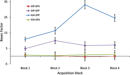
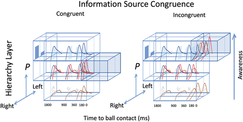
Figure 10. Hierarchical Information Integration Model of Skilful Anticipation (HIIMSA). The HIIMSA model depicts how prior shot outcome probabilities information may be integrated with kinematic shot direction information during a left to right direction decision about a shot outcome. An example of congruent information integration is presented in the left half of the figure (shot outcome probability—rightward shot, kinematic information—rightward shot) and incongruent information integration in the right side (shot outcome probability—rightward shot, kinematic information—leftward shot). Shot outcome probability (9 right, 2 left) is represented in the blue bars in the top layer of the hierarchy and forms the initial top-down prior belief about the actual shot outcome before the shot has begun. The bottom layer represents the sensory evidence (i.e. likelihood) from the kinematic information about a shot outcome over time. Note the left-right probability changes over time as the shot evolves toward ball contact, with a higher peak representing greater probability and the skewness of the distribution curve representing the left-right shot direction. The kurtosis representing the certainty. Initially, the middle layer represents the integration of sensory evidence (i.e. The likelihood, brown distribution line) and the shot outcome probability (i.e. prior, blue distribution line) forming the posterior probability (red distribution lines). As shots evolve over time toward ball racket contact (see millisecond values before ball contact) the previous posterior probability distribution forms the subsequent prior distribution, which could be determined by pick up of kinematic information from a fixation for example. This new sensory evidence is then integrated with the new prior to form the new posterior probability for each information pick up iteration. In the case of congruent information, a higher posterior probability peak is reached with fewer iterations (i.e. earlier in time, approximately 180 ms). When a response window (i.e. A window in time when a timely response can be initiated, blue shaded box) is reached and the posterior probability is above a decision threshold, a response is initiated. In the case of incongruent information, at 360 ms the kinematic information about shot direction in the sensory evidence conflicts with the shot outcome probability prior, which results in a sufficient amount of prediction error to engage the next upper layer of the hierarchy and is reflected in increased awareness. More iterations are required for the posterior probability to reach the decision threshold. This results in a longer response time for the incongruent case. The sensory evidence at the later stage of the shot carries greater probability and weights more heavily onto the posterior probability and subsequent prior iterations. Effort can drive top-down attentional processes by narrowing the distribution width of the prior and increases the likelihood that there will be mismatch between the sensory evidence and the prior, resulting in increased prediction error and engagement of the higher layers thereby increasing awareness and shifting of the subsequent prior, which may facilitate the acquisition of skill.