Player Activity and Load Profiling with Hidden Markov Models: A Novel Application in Rugby League

Figures & data

Table 1. Selected match and training GPS files—their modalities, drills and drill descriptions along with the number of GPS files, average number of observations (seconds) and corresponding average time per GPS file for each drill in minutes and seconds.

Training modality	Training drill	Drill description	Number of GPS files	Average file length (s)	Average time (min, sec)
Attack	Attack sequence	Game scenario with focus on attack patterns with ball-in-hand	100	516	8 min 36s
	Attack (13v13)	13v13 game with focus on attacking team	100	598	9 min 58s
Conditioning	Broncos	20, 40, 60 meters shuttle runs	100	332	5 min 32s
	Maximal aerobic speed (MAS)	Speed intervals	100	242	4 min 2s
Defense	Cage defense	Goal-line defense without ball-in-hand	100	504	8 min 24s
	Edge defense	Defense-focused drills on left & right edges of pitch	100	544	9 min 4s
Small-sided games	Kick pressure game	13v13 game with focus on executing pressure defense tactics	100	269	4 min 29s
	Pole game		100	268	4 min 28s
Transition	Arm wrestle	Game scenario with transition between attack and defense and specific focus on tackling	100	506	8 min 26s
	Transition game	13v13 game scenario with transition between attack & defense	100	445	7 min 25s
Match		Full match GPS files	210	5618	93 min 38s*

*Average playing time reflects time accumulated during stoppages for injuries as well as some matches that went into extra-time play and is thus greater than 80 minutes.

Figure 1. State distributions, with their parameter estimates and corresponding 95% confidence intervals, and stationary state probability plots for the five-state HMM fitted to the training data and the match data. For turning angle distributions, $\mathit{\sigma }$ refers to an angle concentration parameter inversely related to variance. There was no heart rate data available for the match data, hence the absence of the stationary state probability plot in Panel (b).

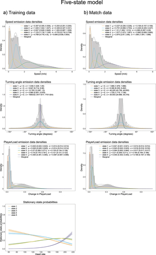
Figure 2. Stationary state probability plots for the five-state HMM, with proportion of match elapsed and score difference as transition probability covariates, fitted to the match data.

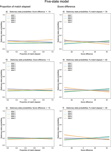
Figure 3. Proportion of time spent in each state for the five-state HMM, across all players for each training modality and the match and predicted match data.

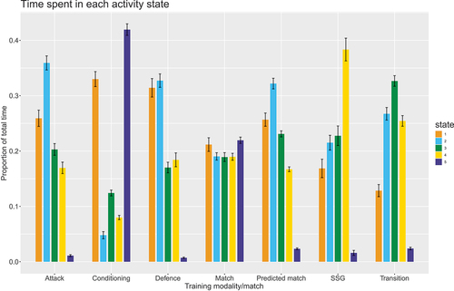
Figure 4. Cumulative time spent in each state (a) and player GPS files (b) for 5-state HMM fitted to training data.

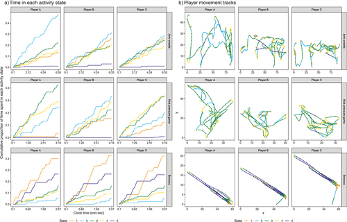
Figure 5. Cumulative time spent in each state (a) and player GPS files (b) for 5-state HMM fitted to match data. For display purposes, only the first 500 observations (500 seconds) of the GPS files are included.

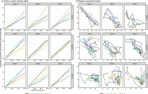
Table A1. AIC values for fitted models.

Model	Data	Num. States	Covariate	AIC	Akaike Weight
m_train3	Training	3		422327	0
m_train3_hr	Training	3	Heart rate	420551	0
m_train5	Training	5		20218	0
m_train5_hr	Training	5	Heart rate	18175	1
m_match3_time	Match	3	Time in game	−237315	0
m_match3	Match	3		−329777	0
m_match3_score	Match	3	Score difference	−330290	0
m_match3_score_time	Match	3	Score difference and Time in game	−330560	1
m_match5	Match	5		−1241251	0
m_match5_time	Match	5	Time in game	−1241547	0
m_match5_score	Match	5	Score difference	−1242116	0
m_match5_score_time	Match	5	Score difference and Time in game	−1242405	1

Figure A1. Examples of (a) GPS les with good quality that were retained and (b) GPS les with poor quality that were removed after visual inspection.

Figure A2. State distributions, with their parameter estimates and 95% confidence intervals for those estimates, and stationary state probability plots for the three-state HMM fitted to the training data (Panel a) and the match data (Panel b). For turning angle distributions, σ refers to an angle concentration parameter inversely related to variance. There was no heart rate data available for the match data, hence the absence of the stationary state probability plot in Panel b.

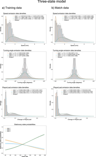
Figure A3. Stationary state probability plots for the three-state HMM, with proportion of match elapsed and score difference as transition probability covariates, fitted to the match data.

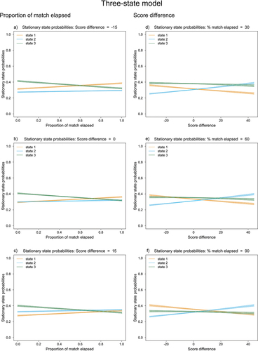
Figure A4. Proportion of time spent in each state for the three-state HMM, across all players for each training modality and for the match and predicted match data. The predicted match file was obtained by using the training model with the overall mean value for the heart rate covariate to predict the Viterbi sequence for each match data player’s GPS file.

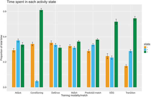
Figure A5. Cumulative time spent in each state (a) and player GPS files (b) for 3-state HMM fitted to training data.

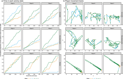
Figure A6. Cumulative time spent in each state (a) and player GPS files (b) for 3-state HMM fitted to match data. For display purposes, only the first 500 observations (500 seconds) of the GPS les are included.

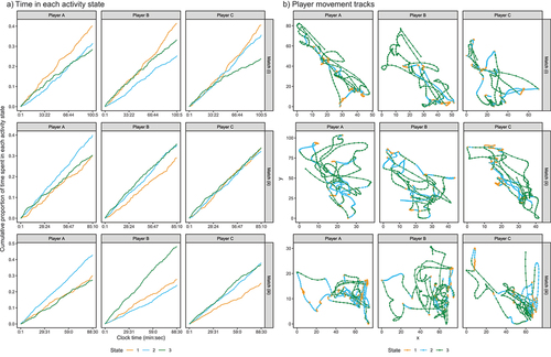
Figure A7. Pseudo-residual plots for three-state HMM fit to the training data.

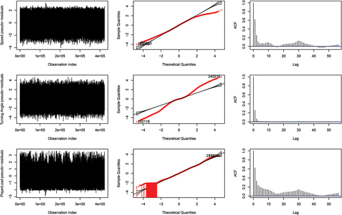
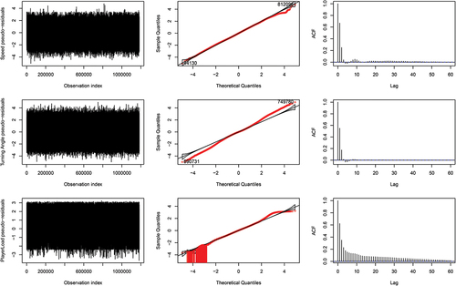
Figure A8. Pseudo-residual plots for five-state HMM fit to the training data.

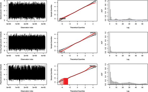
Figure A9. Pseudo-residual plots for three-state HMM fit to the match data.

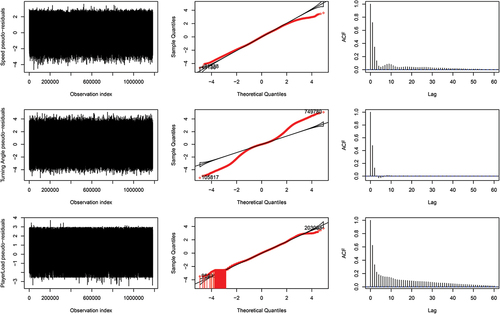
Figure A10. Pseudo-residual plots for five-state HMM fit to the match data.