Figures & data
Figure 1. (a) Rarefaction curves of OTUs. (b) Principal co-ordinates analysis. (c) Partial least squares discriminant analysis.
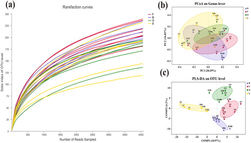
Table 1. Estimates of richness and diversity for operational taxonomic units (OTUs) definition of 97% similarity for twenty-five samples obtained.
Figure 2. (a) Bacterial community structure and distribution at phylum level. (b) Bacterial community structure and distribution at class level.
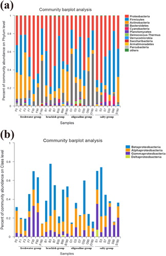
Figure 3. Bacterial community structure and distribution at genus level.
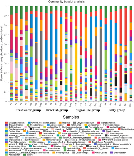
Figure 4. Significantly different relative abundance of dominant bacteria in four groups. Kruskal-Wallis was used to evaluate the importance of comparisons between indicated groups. *P < 0.05, **P < 0.01, ***P < 0.001. (a) At the phylum level. (b) At the genus level.
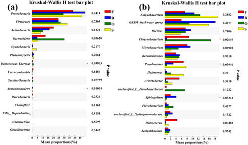
Figure 5. The cladogram of microbial communities. Nodes with different colors represent the microflora that are significantly enriched in the corresponding groups and have significant influence on the differences between groups. Pale yellow nodes indicate the micro-organism groups that have no significant difference in different groups or have no significant influence on the differences between groups.
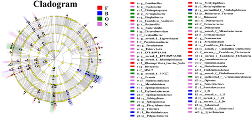
Figure 6. Co-occurrence network analysis for 25 samples. Each node was labelled at the phylum level, shown at the genus level. A connection stands for a strong (Spearman's p > 0.6) and significant (P < 0.05) correlation. The size of each node is proportional to the relative abundance; the thickness of each connection between two nodes (edge) is proportional to the value of Speaman's correlation coefficients. Red and cyan lines indicate positive and negative correlations, respectively. (a) Co-occurrence network analysis for 25 samples. (b) Co-occurrence network analysis of group F samples. (c) Co-occurrence network analysis of group O samples. (d) Co-occurrence network analysis of group S samples.
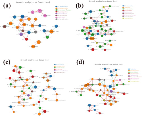
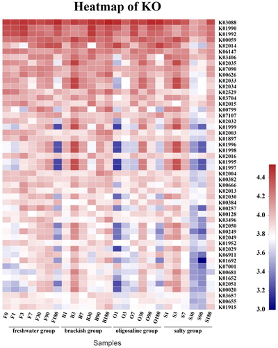
Figure 7. The abscissa is the sample name and the ordinate is the KO number. The color block color gradient is utilized to show the changes in the abundance of different functions in the sample. The legend represents the value represented by the color gradient.