Hyporheic exchange due to in-stream geomorphic structures

Figures & data

Figure 1. Schematic diagram of the custom built flume and other parts of the experimental apparatus. Light gray and blue areas represent sections filled with sand and water, respectively. The dark gray rectangle on the sand bed is a weir set up in the experiment. Sampling port locations, shown schematically.

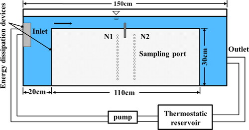
Figure 2. Schematic of the simulation domain and boundaries. Arrows in each figure indicate flow directions. Domains are vertically truncated with only the lowermost portion of the water column and the uppermost portion of the sediments shown. (a) Hydraulics model domain and associated boundaries for the turbulent flow in CFD and groundwater flow in Comsol. L, L₀, H, d, h and L_h are bedform length, distance between weir and boundary, average water depth of overlying water, depth of streambed, the height of the weir, the length of the weir, respectively. (b) For solute transport. Uniform concentration is assumed in the overlying water. The total quantity of solute in the overlying water and the pore water did not vary with time in the flume experiment but the concentration in the overlying water did. For the purpose of simplicity, the solute concentration in the overlying water was kept constant (2.0 g/L). The governing equations are solved sequentially in the following order: (1) RANS k-w, (2) groundwater flow equation, and (3) solute advection–diffusion–dispersion.

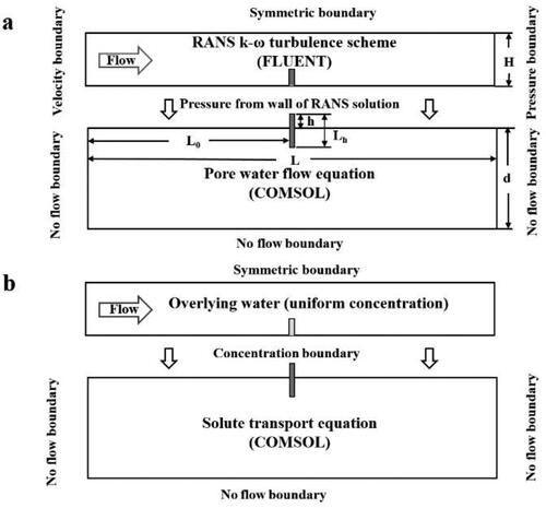
Table 1. Parameters used in the calculation model.

Fluid density ρ (kg·m^−3)	Kinematic eddy viscosity νt (m^2·s^−1)	Porosity θ (%)	Permeability κ (m^2)	Molecular diffusion coefficient Dm (m^2·s^−1)
10^3	1.0 × 10^−6	60	1 × 10^−9	5.0 × 10^−11

Table 2. Accuracy of vertical simulation of the solute concentrations at different monitoring points and periods.

Monitoring sections	Monitoring periods (min)	RMSE (m·s^−1)	R^2	Re (%)
N1	30	0.0073	0.9061	1.08
	60	0.0039	0.9388	0.56
	120	0.0011	0.9688	0.13
	180	0.0022	0.9943	0.25
	300	0.0019	0.9954	0.23
N2	30	0.0021	0.9540	1.64
	60	0.0018	0.9620	1.35
	120	0.0064	0.8413	1.25
	180	0.001	0.9140	0.12
	300	0.0041	0.9122	0.45

Figure 3. (a) Simulated flow rates of the surface water and pore water, as well as (b) interfacial pressures and (c) velocity (vertical velocity). Channel flow is left to right. Thin black lines indicate streamlines. The red arrow lines represent the flow fields.

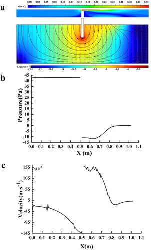
Figure 4. (a) Comparison between the measured (hollow squares) and predicted (red curves) solute concentrations varying with depth. (b) Solute concentration distribution at different times. The color scale for the outputs (b), representing solute concentration; warmer colors: higher concentration, cooler colors: lower concentration. White lines show flow directions (but not magnitude) in the porous media. No vertical exaggeration. Channel flow is left to right.

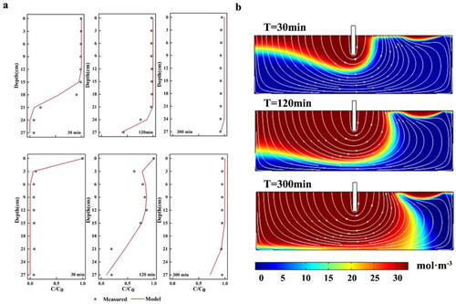
Table 3. Various parameters in the sensitivity analysis.

Factor level	h (cm)	u (m•s^−1)	k (m^2)
1	1	0.04	10^−8
2	2	0.08	10^−9
3	3	0.12	10^−10
4	4		10^−11
5	5		10^−12

Figure 5. (a) Pressure and (b) velocity rate along the sediment-water interface for different weir heights (different colour lines represent schematically different weir heights). The log center is at x = 0.51 m. Simulations of hyporheic fluid flow predict similar patterns upstream and downstream of the weir. Flow in the overlying water column (not shown) is from left to right.

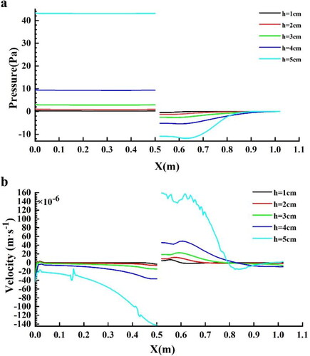
Figure 6. Solute transport fluxes in the streambed for cases with different h at T = 120 min. The color scale for the outputs represents solute concentration; warmer colors: higher concentration, cooler colors: lower concentration. White lines show flow directions (but not magnitude) in the porous media. No vertical exaggeration. Flow in the overlying water column (not shown) is from left to right.

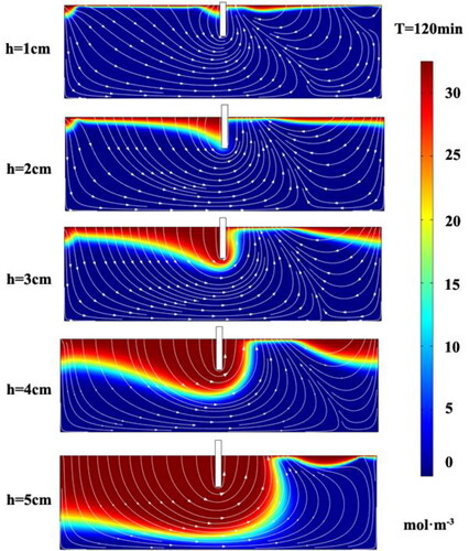
Figure 7. Vertical hyporheic exchange flux (Q), downwelling hyporheic flux (Q_in), upwelling hyporheic flux (Q_out), solute flux (QS), downwelling solute flux (QS_in) and upwelling hyporheic flux (QS_out) in the streambed for cases with different h values. The solid lines represent the hyporheic flow flux; the dashed lines show the solute flux.

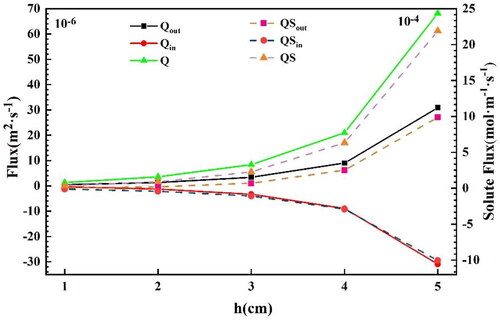
Figure 8. (a) Pressure and (b) vertical hyporheic exchange flux (Q), downwelling hyporheic flux (Q_in), upwelling hyporheic flux (Q_out), solute flux (QS), downwelling solute flux (QS_in) and upwelling hyporheic flux (QS_out) in the streambed for cases with different u values. The solid lines represent the hyporheic flow flux; the dashed lines show the solute flux. (c) Solute transport fluxes in the streambed for cases with different u at T = 120 min. The color scale for the outputs represents solute concentration; warmer colors: higher concentration, cooler colors: lower concentration. White lines show flow directions (but not magnitude) in the porous media. No vertical exaggeration. Flow in the overlying water column (not shown) is from left to right.

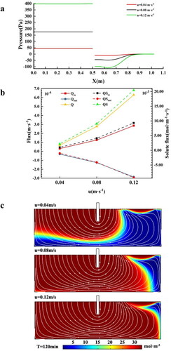
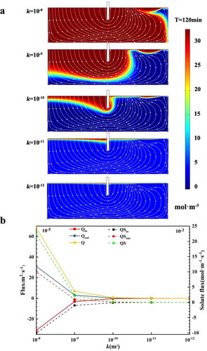
Figure 9. (a) Solute transport fluxes in the streambed for cases with different k at T = 120 min. The color scale for the outputs represents solute concentration; warmer colors: higher concentration, cooler colors: lower concentration. White lines show flow directions (but not magnitude) in the porous media. No vertical exaggeration. Flow in the overlying water column (not shown) is from left to right. (b) Vertical hyporheic exchange flux (Q), downwelling hyporheic flux (Q_in), upwelling hyporheic flux (Q_out), solute flux (QS), downwelling solute flux (QS_in) and upwelling hyporheic flux (QS_out) in the streambed for cases with different k. The solid lines represent the hyporheic flow flux; the dashed lines show the solute flux.