Diagnosis of Dry Eye Disease Using Principal Component Analysis: A Study in Animal Models of the Disease

Figures & data

Figure 1. Histologic changes in inferior lacrimal gland following Concanavalin A

Hematoxylin-eosin stained section of inferior lacrimal gland taken following injection of Concanavalin A. Effacement of normal structure is noted with a severe lymphocytic infiltrate. Only remnants of normal tubuloalveolar structure are visible (yellow arrows); areas of hemorrhagic tissue necrosis with liquefication are seen (red arrow).

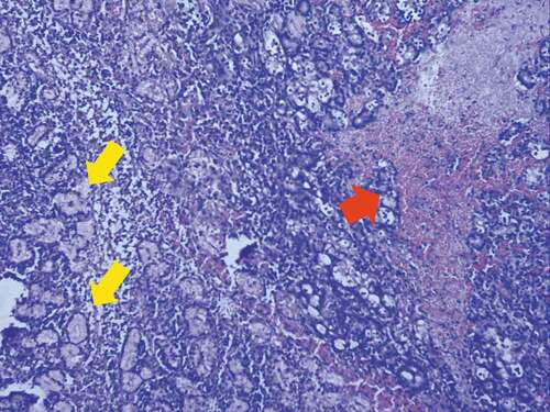
Table 1. Induction of DED in the three study groups

	Surgical (dacryoadenectomy)		Naïve ConA-induced previously untreated		Abnormal ConA-induced previously with DED
	Baseline	Week 1	Baseline	Week 1	Baseline	Week 1
DED test	Mean ± SEM
TBUT, sec	60.0 ± 0.0	5.2 ± 1.2 p ≤ 1x10^−16	60.0 ± 0.3	12.2 ± 2.9 p ≤ 3.2x10^−8	58.5 ± 1.5	29.8 ± 6.9 p = .012
STT, mm	18.3 ± 1.3	9.5 ± 1.6 p ≤ 1x10^−4	14.6 ± 0.4	11.7 ± 1.3 p ≤ 0.044	15.5 ± 0.9	9.0 ± 1.5 p = .0009
TOsm, mOsm/L	291.3 ± 3.7	315.8 ± 2.9 p ≤ 1x10^−5	299.7 ± 1.3	309.2 ± 2.7 p ≤ 0.015	297.2 ± 3.3	297 ± 5.5 p = .83
RB score (NEI, mod)	0.0 ± 0.0	5.6 ± 0.5 p ≤ 1x10^−7	0.0 ± 0.0	5.3 ± 0.6 p ≤ 1.2x10^−5	4.1 ± 0.6	5.6 ± 1.5 p = .12

All statistical comparisons are to the corresponding baseline values

Figure 2. Principal Component Bi-Plots for surgical model of DED

A: Biplots of PC1 vs PC2 (left) and PC1 vs PC3 (right) provide the best meaningful separation of the data without any overlap between Baseline (normal eyes, grey circles) and DED (black circles). Red triangles show the direction and magnitude for the contribution of active variables used to generate the PC axes. The light blue dashed line represents the mathematically defined cutoff for normal versus DED states.

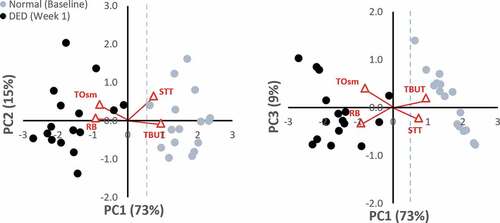
Table 2. Spearman correlation coefficients between DED parameters one week after its induction

	Surgical	Naïve ConA	Abnormal ConA
TBUT/STT	0.539 ^a	0.363 ^c	0.487 ^a
TBUT/TOsm	−0.675 ^a	−0.484 ^b	−0.244 ^c
TBUT/RB	−0.869 ^a	−0.847 ^a	0.019 ^c
STT/TOsm	−0.408 ^b	−0.472 ^b	−0.059 ^c
STT/RB	−0.572 ^a	−0.409 ^c	0.006 ^c
TOsm/RB	0.687 ^a	0.624 ^a	0.115 ^c

The statistical significance of these correlations was: ^a, p < 0.0001–0.005; ^b, p ≤ 0.04; c, not significant.

Table 3. Relative contribution of the variables to principal components (%)

Clinical parameter	PC1	PC2	PC3	PC4
TBUT	30.5	0.7	11.6	57.3
STT	18.4	68.3	13.0	0.4
TOsm	22.2	30.2	46.7	1.0
RB score	28.9	0.8	28.8	41.4

Figure 3. Variance for the surgical model of DED. The eigenvalues and explained variation for each of the four principal components (PC) is shown. The red line at the top depicts the cumulative variability explained, with the variability of each successive PC being added to that of the preceding one, reaching 100% with PC4. The majority of total variation (>70%) is explained by the first component

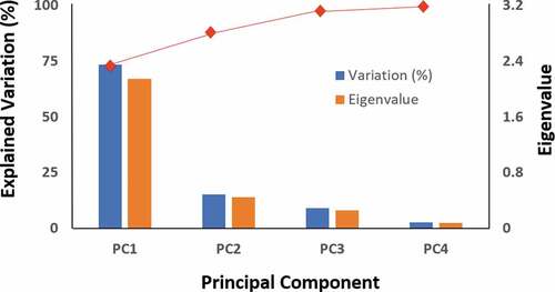
Figure 4. Principal Component Bi-Plots for the ConA groups

a: Biplots of PC1 vs PC2 (left) and PC1 vs PC3 (right) of the Normal ConA group show complete separation of eyes without overlap between normal (Baseline, grey circles) and DED induced in previously untreated eyes using ConA (black circles). b: Biplots of PC1 vs PC2 (left) and PC1 vs PC3 (right) for the Abnormal ConA group show incomplete separation with overlap between Baseline (grey squares) and DED induced in previously treated eyes using ConA (black squares). Although the baseline group appeared normal based on individual parameters, PCA shows this as not normal, no longer having a linear distribution and now occupying a position further to the left along PC1 (the DED side). In both A and B, the red triangles indicate the direction and magnitude of the active variables that generated the PC axes. The light blue dashed line represents the mathematically defined cutoff for normal versus DED states derived from the surgical model.

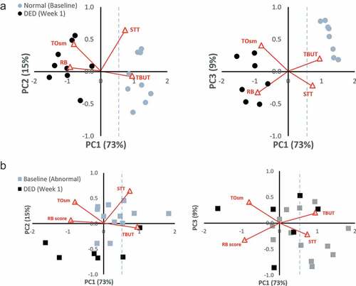
Table 4. P values for individual clinical test parameters and PC scores

Comparison groups	TBUT	STT	TOsm	RB score	PC1
Surgical Baseline vs Surgical DED	2.8x10^−17	5.1x10^−5	6.7x10^−6	3.5x10^−8	2.3x10^−11
Naïve ConA Baseline vs Naïve ConA DED	3.2x10^−8	0.04	0.01	1.2x10^−5	8.2x10^−7
Abnormal ConA Baseline vs Abnormal ConA DED	1.6x10^−5	9.3x10^−4	0.98	0.21	0.02
Abnormal ConA Baseline vs Surgical Baseline	0.33	0.09	0.24	9.3x10^−8	7.3x10^−6